Atomic Orbitals Visualizations

The visualization of atomic orbitals and orbital information is an important enough topic in chemistry and physics to warrant specific attention. Contour plots and surface plots are two popular ways of visualizing a function of two variables, $f(x,y)$, are as a contour plot and as a "three dimensional" surface plots. This work will try various libraries such as Matplotlib, NumPy, and SymPy that creates these types of plots, used some atomic orbital wavefunctions as reference.

Prior knowledge

• Quantum numbers ($$n(principal), l(angular/momentum), ml(magnetic), ms(spin)$$)
• Electron wavefunctions (Atomic orbitals)
• Radial and Angular contributions to the wavefunctions

Electron Wavefunctions (Atomic Orbitals)

Atomic orbitals are describe by a wavefuntion, $$\Psi(n, l, m)$$, which is the product of the radial wavefuntion, $$R_{n, l}(r)$$, and the angular wavefunction, $$Y_{l, m}(\theta, \phi)$$. Each atomic orbital has a different wavefunction $\Psi$, but they sometimes share common radial wavefunctions.

$\Psi_{(n,\; l,\; m)}\;=\;R_{n,\;l}(r)\;\times\;Y_{l,\; m}(\theta,\; \phi)$

The wavefunctions ($\Psi$) is independent of the direction. The radial wavefunction($R$) depends upon the principal ($n$), and angular ($l$). The angular wavefunction describes the direction of the orbital with respect to the sperical coordinate angles and depends upon the angular ($l$) and magnetic ($$m, or, ml$$) quantum numbers.

P11.1 Case study: Atomic Orbital (wavefunctions)

The wavefunction for 2s and 2p orbitals. In polar coordinates:

$$\Psi_{2s}\;=\;N(2-r)e^{-r/2}$$

$$\Psi_{2p}\;=\;N're^{-r/2}\;cos\;\theta$$

Where, $\Psi_{2s}$ and $\Psi_{2p}$ are the wavefunctions for an electron in the 2s and 2p orbitals. $N$ and $N'$ are normalization constants, ensuring the total probability of finding the electron somewhere in space is equal to one. $r$ is radial distances from the nucleus in spherical polar coordinates. $cos;\theta$ is the polar angle (angle from the positive z-axis).

Practically, we evaluate the wavefunctions for polar angles in the range $-\pi\leq0\leq\pi$ to cover the whole of this plane. We will use NumPy and matplotlib for solve this case.

The key arguments:

• np.meshgrid: the coordinate arrays for function
• plt.contour: to make contour plot of the radial distribution function, $r^{2}|\Psi|^{2}$
• plt.axis('square'): forces the plot's aspect ratio to be equal, useful for geometric plots
• plt.axis('off'): turns off the axis lines, tick, and labels (clean visualizations)
• linestyle and linewidth: control the pattern and thick of the line
• plt.contourf: creates filled contour plots, commonly used for visualizing scalar fields (probability densities, electron orbitals).

# use NumPy and Matplotlib
import numpy as np
import matplotlib.pyplot as plt

r = np.linspace(0, 12, 100)
theta = np.linspace (-np.pi, np.pi, 100)
R, theta = np.meshgrid(r, theta)

def psi_2s(r, theta):
    """ Return the value of the 2s orbital wavefunction.

    This orbital is spherically-symmetric so does not depend on the angular coordinates theta or phi. The returned wavefunction is not normalized.

    """
    return (2-r) * np.exp(-r/2)

# To make a contour plot of the radial distribution we can use plt.contour
X, Y = R * np.cos(theta), R * np.sin(theta)
Z_2s = R **2 * psi_2s(R, theta)**2

# Matplotlib will not necessarily set the aspect ratio
plt.contour(X, Y, Z_2s, cmap='jet') # use popular 'jet' colormaps
plt.title(r'$\mathbb{R}\;[\Psi_{2s}]$')
plt.axis('square')
plt.axis()
plt.xlabel(r'$x$-position [a.u.]')
plt.ylabel(r'$y$-position [a.u.]')
plt.savefig('Radial Wavefunctions 2s orbital.svg', bbox_inches='tight')
plt.show()

# use NumPy and Matplotlib
import numpy as np
import matplotlib.pyplot as plt

r = np.linspace(0, 12, 100)
theta = np.linspace (-np.pi, np.pi, 100)
R, theta = np.meshgrid(r, theta)

def psi_2pz(r, theta):
    """ Return the value of the 2pz orbital wavefunction.

    This orbital is cylindrically-symmetric so does not depend on the angular coordinate phi. The returned wavefunction is not normalized.

    """
    return r * np.exp(-r/2) * np.cos(theta)

Z_2pz = R **2 * psi_2pz(R, theta)**2

plt.contour(X, Y, Z_2pz, cmap='jet')
plt.title(r'$\mathbb{R}\;[\Psi_{2p}]$')
plt.axis('square')
plt.xlabel(r'$x$-position [a.u.]')
plt.ylabel(r'$y$-position [a.u.]')
plt.savefig('Radial Wavefunctions 2p orbital.svg', bbox_inches='tight')
plt.show()

P11.2 Case study: Radial wavefunctions

The radial wavefunctions ($R$) are independent of direction, they can be represented effectively on a simple 2D plot. We can use SymPy library includes a funtion R_nl(), this function takes the principal quantum number (n), angular momentum number ($l$), radius Bohrs (r), and atomic number (Z).

R_nl(n, l, m, r, Z=1)

We can calculate the radial wavefunction for any hydrogen-like atomic orbital such as the 2p orbitals (n = 3, and l = 1) at 4.0 Bohrs. To get a float answer, SymPy prefer use the evalf() method.

import sympy
from sympy.physics.hydrogen import R_nl

R_nl(3, 1, 4.0, Z=1).evalf()

0.0425138097805085

P11.3 Case study: Radial wave and Probability density

We can convert $R_nl$ function to a function that can accept an array using the lambdify() method.

Prior knowledge

• Radial wavefunction, $R_{n, \ l} (r)$

  The radial part of the wavefunction, $R_{n, l}(r)$ gives the radial variation of $\Psi$. $R_{n, l}(r)$ defines how the wavefunction depends on the distance of the electron from the nucleus (the radius).

• Probability density, $R^{2} r^{2}$

  The electron probability density can be found by calculating $R^{2}$ where $R$ is the radial wavefunction, and the radial probability is $R^{2} r^{2}$ where $r$ is the distance from the nucleus. Just like in the particle-in-a-box model, the square of the wavefunction is proportional to the probability of finding a particle (electron) at some point in space. The square of the radial part of the wavefunction is called the radial distribution function $4\pi^{2}(R_{n, l}(r))^{2}$, and its describes the probability of locating the electron at some distance $r$ away from the nucleus.

  Conclude, that $R^{2}r^{2}$ gives the probability per unit volume, while $4\pi^{2}(R_{n, l}(r))^{2}$ gives the total probability of finding the electron within a spherical sheel of thickness $dr$ at distance $R$.

  The radial probability is $R^{2}r{2}$. The reason we multyply the probability density by the square of the radial wavefunction, $r^{2}$, is to account for the greater surface area of a sphere ($A_{sphere} = 4\pi r^{2}$) the larger the radius. We are effectively carrying out the calculation depicted below. We divide the sphere surface area by $4\pi$ to normalize the integration, making the probability over all space total to 1.

import numpy as np
import matplotlib.pyplot as plt
import sympy
from sympy.physics.hydrogen import R_nl
import math

r = sympy.symbols('r')
R_3p = sympy.lambdify(r, R_nl(3, 1, r, Z=1), modules='numpy') # use lambdify() method
radii = np.linspace(0, 30, 200)

fig = plt.figure(figsize=(28, 6))

ax1 = fig.add_subplot(1, 4, 1)
ax1.plot(radii, R_3p(radii), color='C0')
ax1.set_xlabel(r'$r/a_{0}\;(Bohrs)$')
ax1.set_ylabel(r'The Radial Wavefunction, $R(r)$')
ax1.set_title('3p Radial function')
ax1.hlines(0, 0, 30, color='r', linestyle='dashed')

ax2 = fig.add_subplot(1, 4, 2)
ax2.plot(radii, R_3p(radii)**2 * radii**2, color='C2')
ax2.set_xlabel(r'$r/a_{0}\;(Bohrs)$')
ax2.set_ylabel(r'Radial Probability, $R^{2}\;r^{2}$')
ax2.set_title('3p Radial probability')

ax3 = fig.add_subplot(1, 4, 3)
ax3.plot(radii, 4 * sympy.pi * radii**2 * R_3p(radii)**2 * radii**2, color='C1')
ax3.set_xlabel(r'$r/a_{0}\;(Bohrs)$')
ax3.set_ylabel(r'Radial Probability, $4\pi r^{2}R^{2}\;(r)$')
ax3.set_title('3p Radial probability distribution')

ax4 = fig.add_subplot(1, 4, 4)
ax4.plot(radii, 4 * sympy.pi * radii**2, color='C3')
ax4.set_xlabel(r'$r/a_{0}\;(Bohrs)$')
ax4.set_ylabel(r'Surface Area / $4\pi r^{2}$')
ax4.set_title(r'Sphere Surface Area Over $4\pi$')
plt.savefig('Probability density 3p orbital.svg', bbox_inches='tight')
plt.show()

P11.4 Case study: Multiple plots

We can use the radial plots to compare the radial probability of multiple different orbitals on the same axes. For example create the radial probability use the valence electron configurations of Cr and Cu.

import sympy as sp
import numpy as np
import matplotlib.pyplot as plt

import sympy
from sympy.physics.hydrogen import R_nl

# Use lambdyfy and SymPy
# create SymPy sumbol
r = sympy.symbols('r')

# Create a numpy function to define radial function (R_nl)
R_3s = sympy.lambdify(r, R_nl(4, 0, r, Z=1), modules='numpy')
R_3p = sympy.lambdify(r, R_nl(4, 1, r, Z=1), modules='numpy')
R_3d = sympy.lambdify(r, R_nl(3, 2, r, Z=1), modules='numpy')

radii = np.linspace(0, 45, 200)

# create plot
plt.plot(radii, R_3s(radii)**2 * radii**2, label = '4s')
plt.plot(radii, R_3p(radii)**2 * radii**2, label = '4p')
plt.plot(radii, R_3d(radii)**2 * radii**2, label = '3d')
plt.xlabel(r'$r/a_{0}\;(Bohrs)$')
plt.ylabel(r'Radial Probability, $R^{2}\;r^{2}$')
plt.title('Multiple plots of 4s, 4p, 3d orbitals')
plt.savefig('Multiple plots of 4s, 4p, and 3d orbitals.svg', bbox_inches='tight')
plt.legend();

P11.5 Case study: Angular Wavefunctions, $Y_{l, m}(\theta, \phi)$

The angular contribution to the wavefunction, $Y_{l, m}(\theta, \phi)$, describes the wavefunction's shape, or the angle with respect to a coordinate system. To describe the direction in space, we use spherical coordinates that tell us distance and orientation in 3-dimensional (3D) space. There ae three spherical coordinates: $r, \phi,$ and $\theta$.

$$Y_{l,\;m}(\theta,\;\phi)=(\frac{1}{4\pi})^{1/2}\;y(\theta,\;\psi)$$

Where $r$ is the radius, or the actual distance from the origin. $\phi$ and $\theta$ are angle. $\phi$ is measured from the positive x axis in the xy plane and maybe between 0 and $2\pi$. $\theta$ is measured from the positive z-axis towards the xy plane and may be between 0 and $\pi$.

$Y_{l, m}(\theta, \phi)$, is slightly more difficult to describe than the radial contribution was. This is partly because $Y_{l, m}(\theta, \phi)$ contains imaginary numbers, which have no real, physical meaning.

Angular wavefunction visualizations

There are multiple conventions for spherical coordinates. We will use the SciPy/SymPy convention of using theta ($\theta$) for the azimuthal (direction on xy-plane) and phi ($\phi$) as the polar angle (angle for the positive z-axis) for plotting the angular wavefunctions.

we try to plot the $d_{z^{2}}$ orbital by coding the angular wavefunction expression by hand.

Step 1: create a mesh grid of angles

• theta: polar angle (0 to $\pi$), measured from the z-axis.
• phi: azimuthal angle (0 to $\pi$), measured around the xy-plane.
• np.meshgrid: create a grid of all possible ($\theta,;\pi$) pairs, so we can evaluate functions across the whole.

Step 2: convert spherical coordinates to Cartesian

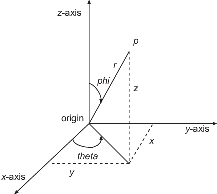
These are the standard spherical to Cartesian transformations with radius $r$ = 1.

• x = r x sin (phi) x cos (theta)
• y = r x sin (phi) x sin (theta)
• z = r x cos (phi)

Step 3: Define the angular wavefunction Refererence: Table of Spherical Harmonics Formula for complex spherical harmonics ($l=2$)

$$Y_{2}^{0}(\theta,\;\phi)=\frac{1}{4} \sqrt{5}{\pi}\;(3 cos^{2}\;\theta - 1)$$

Step 4: Scale the sphere by the wavefunction

• The sphere coordinates are multiplied by the wavefunction value.
• This "inflates" or "deflates" the sphere depending on the angular probability distribution.
• The result is a 3D shape that represents the orbital's angular dependence.

Step 5: Plot the surface

• ax.plot_surface: Creates a 3D plot of the orbital surface
• cmap: applied a color gradient

import numpy as np
import matplotlib.pyplot as plt

import sympy
from sympy.physics.hydrogen import R_nl

# generate mesh grid of theta and phi values
theta, phi = np.meshgrid(np.linspace(0, np.pi, 51),
                         np.linspace(0, 2*np.pi, 101))

# convert angles to xyz values of a sphere, r = 1
x = np.sin(theta) * np.sin(phi)
y = np.sin(theta) * np.cos(phi)
z = np.cos(theta)

# multipy xyz values by angular wavefunction
dz2 = np.sqrt((5/16) * np.pi) * (3 *np.cos(theta)**2 - 1)
X, Y, Z = x * dz2, y * dz2, z * dz2

# Plot the surface
fig = plt.figure(figsize = (10, 8))
ax = fig.add_subplot(1, 1, 1, projection='3d')
ax.plot_surface(X, Y, Z, cmap='jet')
ax.set_title(r'$Spherical\;Harmonics\;d_{z^{2}}\;orbital\;/\;Y_{2}^{0}\;(\theta,\;\phi)$')
ax.set_xlabel(r'$x$-axis [a.u.]')
ax.set_ylabel(r'$y$-axis [a.u.]')
ax.set_aspect('equal')
plt.savefig('Angular Spherical Harmonic dz^2 .svg', bbox_inches='tight')
plt.show()

P11.6 Case study: Polar Plots, $Y_{l}^{m}(\theta)$

We can visualize the angular component of wavefunction in 2D using polar plot, but we can only visualize one angle at a time. We will visualize theta and leave phi fixed, because we are only visualizing in 2D and not sweaping around the phi angles.

Visualization of the spherical harmonics

The Laplace spherical harmonics $\large{Y_{l}^{m}}$, can be visualized by considering their nodal lines. Analytic expression for the first few orthonormalized Laplace spherical harmonics $\large{Y_{l}^{m}}:\large{S^{2}} \rightarrow \mathbb{C}$ that use the Condon-Shortley phase convention.

Step 1: Quantum numbers setup

• l and m: l is orbital angular momentum quantum number, m is magnetic quantum number.

Step 2: Symboliz variables

• azmuth: correspond to the azimuthal angle $\phi$.
• polar: correspond to the polar angle $\theta$.

Step 3: Spherical harmonic function

• Z_lm(l, m, polar, azmuth): the spherical harmonic function ($Y_{l}^{m}(\theta, \phi)$).
• sympy.lambdify: converts the symbolic expression into a numerical function f that can be evaluated with NumPy arrays.
• f(theta, phi): gives numerical values of the spherical harmonic.

Step 4: Angle sampling

• These represent aimuthal angles
• Creates 200 evenly spaced values between 0 and $2\pi$.

Step 5: Polar plot setup

• polar=True: means the axes are circular, with angles radiating outward.

Step 6: Plotting the spherical harmonic slice

• th: sweeps through azimuthal angles
• np.abs: plots the absolute value of the spherical harmonic.

Step 7: Orienting the plot

• Sets the zero angle (0 radians) to point north (up) instead of the default east (right).

import numpy as np
import matplotlib.pyplot as plt

import sympy
# delete this cell and replace with actual Z_lm after next SymPy release
from sympy.functions.special.spherical_harmonics import Znm
def Z_lm(l, m, phi, theta):
    return Znm(l, m, theta, phi).expand(func=True)

# Quantum numbers
l, m = 2, 0

# Define symbolic variables
azmuth, polar = sympy.symbols('azmuth polar')

# Use SimPy spherical harmonics function
# Z_lm(l, m, theta, phi) gives the spherical harmonics
f = sympy.lambdify((polar, azmuth), Z_lm(l, m, polar, azmuth), modules='numpy')

# Sample Azimuthal angles
th = np.linspace(0, 2 * np.pi, 200)

# Polar plot
fig = plt.figure()
ax = fig.add_subplot(111, polar=True)

# Evaluate spherical harmonic at polar angle = 0
ax.plot(th, np.abs(f(0, th)))
ax.set_title(r'$d_{z^{2}}\;orbital\;/\;Y_{l}^{m}(\theta)$')

# Orient 0 degress to north
ax.set_theta_zero_location('N')
plt.savefig('Angular polar 3d^2 orbital.svg', bbox_inches='tight')

P11.7 Case study: Complete Wavefunction, $\psi(n, l, m) = R(n, l)Y(l, m)$

Before we knew about quantum physics, humans tought that if we had a system two small objects, $x_{1}$ and $x_{2}$. In the Quantum world, based on Schrodinger's 1925 theory of quantum physics, the objects become the complex number $\psi(x_{1}, x_{2}$. In this work, we will visualize both angular and radial components together ($\psi$) which is again the product of the radial, $R(n, l)$ and angular, $Y(l, m)$ wavefunctions.

Orbitals have no edge, so there are multiple ways of representing orbitals, including:

• contour plots
• isosurfaces
• surface plots
• scatter plots
• translucent 3D plots.

To visualize the orbitals we need the probability density, P, of the atomic orbital, which is proportional to the product of a wavefunction, $\psi$, and its complex conjugate, $\psi^{*}$ or the square of the absolute value of a wavefunction.

$$P\;=\;\psi*\psi\;=\;|\psi|^{2}$$

Strategy: we use the SymPy Psi_nlm() function.

Defining the key arguments

• lambdify: converts the symbolic expression into a fast numerical function.
• wf_sym: a symbolic expression for the hydrogenic wavefunction.
• theta_vals: a NumPy array of sampled polar angles $\theta$.
• np.arccos: the inverse cosine function, because the orbital plot would be biased (too many points near the polar or equator).
• prob_dens: the probability density at each sampled point
• wf(): evaluates the wavefunction numerically at each sampled ($r,;\theta,;\phi$)
• norm_prob: normalized probability density.
• mask: a boolean selecting which points to keep.
• is_pos: a boolean array indicating the sign of the wavefunction, positive values = one lobe (red), and negative value (blue). Used for coloring lobes.

The 3d orbital scatter plots

Quantum number and angular and spherical coordinates n = 3(principal), l = 2 (d-orbital), m = 0 (aligned along z)

• polar is the polar angle $\theta$, then multiplying by sin(0) in the Cartesian conversion. That effectively sets x = 0 always, collapsing visualization into the yz-plane.
• for spherical coordinates, we need both, $\theta$ (polar angle, 0 to $\pi$), $\phi$ (azhimutal angle, 0 to 2$\pi$).

  # 3d orbital
import numpy as np
import matplotlib.pyplot as plt

import sympy
from sympy.physics.hydrogen import Psi_nlm

# Define symbols
r, polar = sympy.symbols('r, polar')

# 3d orbital wavefunction (n=3, l=2, m=0)
wf_sym = Psi_nlm(3, 2, 0, r, 0, polar)
wf = sympy.lambdify((r, polar), wf_sym, modules='numpy')

# generate random coordinates
rng = np.random.default_rng(seed=21)
n_points = 500000
r = 30 * rng.random(size=(n_points))
polar = 2 * np.pi * rng.random(size=(n_points))

x = r * np.sin(polar) * np.sin(0)
y = r * np.sin(polar) * np.cos(0)
z = r * np.cos(polar)

# normalize and create mask
prob_dens = np.abs(wf(r, polar))**2
norm_prob = prob_dens / prob_dens.max()
mask = norm_prob > rng.random(n_points)

# plt.plot (x[max], y[max])
fig = plt.figure(figsize = (5, 5))
ax = fig.add_subplot(1, 1, 1)
is_pos = wf(r, polar)[mask] > 0
ax.scatter(y[mask], z[mask], s=0.5, c=is_pos, cmap='coolwarm')
ax.set_xlabel(r'$r/a_{0}\;(Bohrs)$')
ax.set_ylabel(r'$r/a_{0}\;(Bohrs)$')
ax.set_title(r'$3d\;Scatter\;orbital\;(\psi)$')
plt.savefig('Scatter 3d orbital.svg', bbox_inches='tight')

The 3d orbital contour plots

A second way to visualize orbitals is through a contour plot. Here we calculate the probability in a mesh of locations and provide the plt.contour function with the location and probabilities. We use spherical conversion:

$$r=\sqrt{Y^{2}\;+\;Z^{2}},\; \theta=arcoss(\frac{Z}{r})$$

The key arguments:

• Y and Z: are 2D arrays representing coordinates (200 x 200 points spanning -20 to 20 Bohr radii)
• r: radial distance from nucleus.
• polar: polar angle $\theta$ (angle from z-axis).
• f(r, polar): computes probility density numerically.
• r = np.sqrt(Y^2 + Z^2): radial distance from origin.
• polar = arctan(Y / Z): polar angle approximation.
• plt.contour: draw contour lines of constant probability density.

# 3d orbital
import numpy as np
import matplotlib.pyplot as plt

import sympy
from sympy.physics.hydrogen import Psi_nlm

# Create a grid of points
Y, Z = np.meshgrid(np.linspace(-20, 20, 200),
                    np.linspace(-20, 20, 200))

# Define symbolic variables
r, polar = sympy.symbols('r polar')

# Build the wavefunction
wf = Psi_nlm(3, 2, 0, r, 0, polar)

# Convert to numerical function
f = sympy.lambdify((r, polar), wf * sympy.conjugate(wf), modules='numpy')
                   
# Convert grid coordinates to spherical
polar = np.arctan(Y / Z)

# calculate probability density
r = np.sqrt(Y**2 + Z**2)
prob = np.abs(f(r, polar))**2

# plot contours
plt.contour(Y, Z, prob, levels=[1e-9, 3e-9, 5e-9, 1e-8, 5e-8, 1e-7, 3e-7, 5e-7], cmap='jet')
plt.colorbar()
plt.xlabel(r'$r/a_{0}\;(Bohrs)$')
plt.ylabel(r'$r/a_{0}\;(Bohrs)$')
plt.title(r'$3d\;Contour\;orbital\;(\psi)$')
plt.savefig('Contour 3d orbital.svg', bbox_inches='tight')