The main aim of this study is to predict the probability of an attack being successful based on different factors. There are several factors which aid the success of an attack like the number of hours of an attack, the time of the day, and the presence of security are among other factors. With this model we will have a deeper understanding of the occurrences of these attacks; which, will help the relevant authorities to stop them or minimize their occurrences. This study will also focus on determining the most rampant type of attacks in the world. This study will be aimed at solving the following research objectives:
- To determine the most frequent attack type.
- To determine if there is significance difference in the number of hours taken between those attacks that were successful and those that failed.
- To determine if there is a relationship between the wounds incurred during an attack and number of hours the attack occurred.
- To determine if there is significance difference in the number of hours taken between different types of attacks
- To determine the impact of other factors on the success of the attack.
For the purpose of this study we extracted data from Kaggle using the following URL: https://www.kaggle.com/START-UMD/gtd. This data was collected by the Global Terrorism Database (GTD) which is an open-source database including information on terrorist attacks around the world from 1970 through 2017. The GTD includes systematic data on domestic, as well as, international terrorist incidents that have occurred during this time period, and now includes more than 180,000 attacks. The database is maintained by researchers at the National Consortium for the Study of Terrorism and Responses to Terrorism (START), headquartered at the University of Maryland. This dataset contains more than 135 variables, but we were only interested in a few variables. The variables of interest in this study were as follows:
nhours: the number of hours under attack ndays: number of days under attack Ransom: the reason amount being requested Success: whether the attack was successful or not Type of attack: the type of attack imonth: The month that the attack happened iyear: the year that the attack happened iday: the day that the attack happened specificity: location
We will use descriptive statistics to have an overview of how the data looks and determine the kind of relationships that exist in the dataset. We will use data visualization to chart the data in a form that is easy to understand and interpret. Regression analysis(relationships between variables), two sample t test(determine if there is significane for two variables), correlation analysis(determine relationship between two variables) and one way Anova(comparing more than two variables) will be used to solve objective 2, 3, 4 and 5. The results of this study are as shown below.
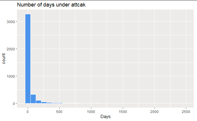
Figure 1 The variable number of days in which a place, building or a person was under attack was skewed to the right. This is shown by the results in figure 1 above where the tail of the histogram was longer to the right.
#Code:
# Histogram of number of days under attack
library(ggplot2)
ggplot(mydata, aes(x = ndays)) +
geom_histogram(fill = "cornflowerblue", color = "white") +
labs(title="Number of days under attcak",x = "Days")
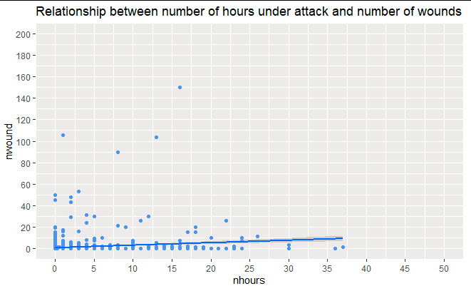
Figure 2 The scatter plot in figure 2 above indicates the relationship between the number of hours under attack and the number of wounds a person incurred. There was a positive relationship between the number of wounds incurred by a person and the number of hours the person was being attacked. To determine the nature and strength of the relationship we will conduct pearson correlation test.
#Code:
#ggplot(mydata,
    aes(x = nhours, y = nwound)) +
geom_point(color="cornflowerblue")+
    scale_x_continuous(breaks = seq(0, 50, 5), limits = c(0, 50))+
scale_y_continuous(breaks = seq(0, 200, 20), limits = c(0, 200))+
geom_smooth(method = "lm")+
    labs(title = "Relationship between number of hours under attack and number of wounds")
To determine the most frequent attack type, a bar chart is the most appropriate tool to use. This is because, the variable type of attack is a categorical variable and bar chart is the most appropriate to represent the difference between the groups found in the variable.
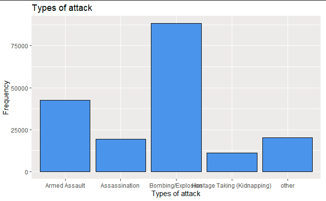
Figure 3 above indicates the type of attack that were being witnessed and the frequency at which, they were happening. Based on this results, bombing and explosion attacks were the most rampant ones followed by armed assault, other kind of attacks, and assassination. There were very few attacks which are categorized as hostage (kidnapping) that were witnessed.
#Code:
#ggplot(mydata, aes(x = Form_attack)) +
  geom_bar(fill = "cornflowerblue",
	   color="black") +
  labs(x = "Types of attack",
       y = "Frequency",
       title = "Types of attack")
To determine if there is significance difference in the number of hours taken between those attacks that were successful and those that failed, two sample t test will be the most appropriate test as the grouping variable success has two groups and nhours is a categorical variable.
# Code: t.test(nhours~success)

	Welch Two Sample t-test

	Data:  nhours by success
	t = -2.7694, df = 155.77, p-value = 0.006299

	Alternative hypothesis: true difference in means between group 0 and group 1 is not equal to 0

	95 percent confidence interval:
	 -12.057453   -2.017913

	Sample estimates:
	Mean in group 0    mean in group 1
	       3.026316       10.063999
The attacks which went on successful had a significantly different number of hours that it occurred (N=10.06) as compared to those which were not successful (N=3.02), df= (155.77) t=-2.7694, p =0.0062. The study rejects the null hypothesis since the p value is less than the significance alpha value of 0.05. Those attacks that went through successfully took longer hours.
To determine if there is a relationship between the wounds incurred during an attack and number of hours the attack occurred, correlation test was the most appropriate test as both the variables are numeric. The correlation results are as follows:
#Code: cor.test (nhours, nwound)

	Pearson's product-moment correlation

	Data:  nhours and nwound
	t = -0.13643, df = 1778, p-value = 0.8915
	Alternative hypothesis: true correlation is not equal to 0
	95 percent confidence interval:
	-0.04968931  	0.04323236
	Sample estimates:
		Cor
	-0.003235459
There was a weak negative correlation between the number of hours a person was under attack and the number of wounds incurred, correlation estimate or r=-0.003, p= 0.8915. The p-value is high because of the r value being so low and negative. We keep the null hypothesis that there is no relationship between hours and wounds.
Analysis of variance is the most appropriate test to determine if there was a significance difference in the number of hours that an attack occurred for different types of attack. This the categorical variable had more than two groups and there was a numeric variable. The results of the test are as shown below:
#Code: a<-aov(nhours~Form_attack)
	summary(a)

		Df     Sum 	Sq Mean    Sq F value   	Pr(>F)
	Form_attack     4   	193668      48417   		5.985 8.73e-05 ***
	Residuals      1932 	15628154    8089
Signif. codes: 0 ‘’ 0.001 ‘’ 0.01 ‘’ 0.05 ‘.’ 0.1 ‘ ’ 1 179754 observations deleted due to missingness
Based on the results from table 2 above, there was a significance code of '***', which is extremely low and therefore there is a significance difference in the number of hours that different attacks occurred.
To determine the impact of different factors on whether an attack will be successful or not, multiple linear regression analysis is the most appropriate test. This is because the response variable has been coded as a numeric variable and there are more than one independent variables. Success is coded as 1 and failures as 0. A positive coefficant estimate indicates that success will increase. Then we use f value together with p value to determine if the whole model is significant.
The results of the model are as shown below:
Call:
	Code: lm(formula = success ~ nhours + Form_attack + specificity)
Residuals:
     Min       	1Q   		Median      	 3Q      		Max
-0.99662  	0.00749  	0.00752  	0.00958  	0.11174
Coefficients:
                                     	Estimate  Std. Error  t value Pr(>|t|)
(Intercept)                             9.883e-01  6.949e-03 142.237  < 2e-16 ***
nhours                                  8.096e-06  2.471e-05   0.328  0.74326
Form_attackAssassination               -1.022e-01  1.987e-02  -5.142 2.99e-07
Form_attackBombing/Explosion           -5.744e-02  1.896e-02  -3.030  0.00248
Form_attackHostage Taking (Kidnapping)  2.054e-03  6.977e-03   0.294  0.76847
Form_attackother                       -2.783e-03  8.268e-03  -0.337  0.73641
specificity                             2.072e-03  1.874e-03   1.106  0.26878

Residual standard error: 0.09769 on 1929 degrees of freedom (179755 observations deleted due to missingness)
			Multiple R-squared:  0.2152,	Adjusted R-squared:  0.1848
			F-statistic: 7.072 on 6 and 1929 DF, p-value: 1.827e-07
The regression model is significant in the prediction of whether an attack will be successful or not based on form of attack, specificity and number of hours, p=1.827e-07, F (6, 1929) = 7.072. The study rejects the hypothesis that the model is insignificant. The model is able to predict 18.48% of the variation in the response variable using the predictor variable.
From the regression model above, nhours has a coefficient estimate of 0.0000809. This indicates that for every unit increase in the number of hours under attack the higher the chance of the attack being successful. The variable attack from hostage taking has a coefficient estimate of 0.0027 compared to assault while assassination has a coefficient estimate of -0.1022. Specificity has a coefficient estimate of 0.00207 in the regression model. This indicates that for every unit increase in the specificity there is a 0.00207 unit increase in an attack being successful.
The code below selects 3 categories and binds them to a dataframe. We take this new frame and run a summary of it to display things like mean. # df<-as.data.frame(cbind(nhours,nwound,ndays)) summary(df) #Describes the basics of wounds, hours, and days.
		Show in New Window
	     nhours           nwound             ndays
	 Min.   :  0.00   Min.   :   0.000   Min.   :   0.0
	 1st Qu.:  0.00   1st Qu.:   0.000   1st Qu.:   1.0
	 Median :  0.00   Median :   0.000   Median :   4.0
	 Mean   :  9.99   Mean   :   3.168   Mean   :  40.6
	 3rd Qu.:  1.00   3rd Qu.:   2.000   3rd Qu.:  18.0
	 Max.   :999.00   Max.   :8191.000   Max.   :2454.0
	 NA's   :179754   NA's   :16311      NA's   :177822
Next we import psych, so we can run the describe function. The table produced displays descriptive statistics of the major numeric variables in the set. For instance, the mean number of days that attacks happened was 9.99.
# library(psych)
  describe(df)

# Descriptive

   		vars   	n    	mean  	 sd     median   trimmed  mad    min     max      range    skew      kurtosis
nhours    1   	1937  	9.99  	90.40      0      0.60    0.00    0       999       999     10.82     115.33
nwound    2  	165380 	3.17  	35.95      0      0.89    0.00    0       8191      8191    174.70    36808.41
ndays     3   	3869  	40.60 	143.68     4      11.31   4.45    0       2454      2454    8.25      89.50

#describe(df) produces - item name, item number, number of valid cases, mean standard deviation, trimmed mean (with trim defaulting to .1),
median (standard or interpolated mad: median absolute deviation (from the median). minimum maximum skew kurtosis standard error.
From this study, it is evident that the most frequent crime in the world is bombing and explosion attacks. Armed assault, other kind of attacks, and assassination were also significantly higher than hostage (kidnapping). This shows how much effort the world community should put in place to curb this kind of attacks which have been the cause of a lot of deaths and destructions in the world. Sensitization of the importance of peace in those areas which have been affected the most and offering those people willing to quite terrorism a pathway to rehabilitation back to the society. The rates of kidnapping in the world were very few. The measures put in place should continue being enforced to curb it even more.
It was also evident that that those attacks which were successful took a much longer time than those that were unsuccessful. This indicates that when there is no intervention during attacks such as, police intervention or the intervention of the public there is a higher likelihood of it being a success. People should have contact people whom they can reach during attacks or the toll number be made more efficient so that the police and security force can be easily notified in case of any attacks. There was a significance difference in the time that different attacks took. The one weakness with one way Anova that was used for this test is that it did not show which groups were significantly different from the other.Another limitation for this study was the presence of many missing values which interferes with the meaningfulness and accuracy of the results. There were many variables that lacked the variable description making it hard to use this variables in the model and for other tests. The reliability of the model was very low this might be attributed to a lot of missing values.
#Resources:

	How to compare means - http://www.sthda.com/english/wiki/comparing-means-in-r

	two sample t test - https://www.youtube.com/watch?v=yF9_SQ8m698
	t-test w/ dplyr - https://www.youtube.com/watch?v=ANMuuq502rE
	how to report t-test - http://www.csic.cornell.edu/Elrod/t-test/reporting-t-test.html

	correlation test - https://www.statology.org/correlation-between-multiple-variables-in-r/
	how to test statistical significance of correlation - https://www.youtube.com/watch?v=e3MNPRQgVgU-5uv4wryI

	Analysis of variance (Anova) - https://www.youtube.com/watch?v=5SIifsW2aKA
	Anova reference book - https://bookdown.org/steve_midway/DAR/understanding-anova-in-r.html
	Interpreting results - https://www.youtube.com/watch?v=D3d89aoWRR4


	# Raw Code:
	---
title: "final2"
author: "chase"
date: "12/7/2021"
output:
  html_document: default
  pdf_document: default
---
knitr::opts_chunk$set(echo = TRUE)

# Reading data into R studio
mydata<-read.csv ("C:/Users/computer/Documents/GitHub/chaseaham.github.io/globalterrorismdb_0718dist.csv")


# removing negative values, there were negative observations like number of hours and days.
mydata[mydata < 0] <- NA
attach(mydata)

# To make the data easier to work with, we create a new data frame called Form_attack where the top 4 forms of of attack from attacktype1_txt in mydata are selected and the remainders are rolled into 'other'.

library(dplyr)
Form_attack<-mydata |>
  select(attacktype1_txt) |>
  mutate(
    type = case_when(
      attacktype1_txt=="Armed Assault" ~ "Armed Assault",
      attacktype1_txt=="Assassination" ~ "Assassination",
      attacktype1_txt=="Hostage Taking (Kidnapping)" ~ "Hostage Taking (Kidnapping)",
      attacktype1_txt=="Bombing/Explosion" ~ "Bombing/Explosion",
      TRUE                      ~ "other"
    )
  )

#Taking one column from the new data frame and merging it back into the original with the name type.
Form_attack<-Form_attack$type

mydata<-as.data.frame(cbind(mydata,Form_attack))
attach(mydata)

# Histogram of number of days under attack
library(ggplot2)
ggplot(mydata, aes(x = ndays)) +
  geom_histogram(fill = "cornflowerblue",
                 color = "white") +
  labs(title="Number of days under attcak",
       x = "Days")

# A point plot with a slope showing the relationship between the number of hours under attack and wounds.
ggplot(mydata,
       aes(x = nhours,
           y = nwound)) +
  geom_point(color="cornflowerblue")+
      scale_x_continuous(breaks = seq(0, 50, 5), limits = c(0, 50))+
  scale_y_continuous(breaks = seq(0, 200, 20), limits = c(0, 200))+
  geom_smooth(method = "lm")+
      labs(title = "Relationship between number of hours under attack and number of wounds")

# To determine the most frequent attack type

ggplot(mydata, aes(x = Form_attack)) +
  geom_bar(fill = "cornflowerblue",
           color="black") +
  labs(x = "Types of attack",
       y = "Frequency",
       title = "Types of attack")

#To determine if there is significance difference in the number of hours taken between those attacks; that were successful and those that failed. We are looking at the p-value or mean and comparing it to the alpha value. P-value is lower than the alpha value, so we reject the null hypothesis. There is a relationship.
t.test(nhours~success)


#To determine if there is a relationship between the wounds incurred during an attack
#and number of hours the attack occurred. The relationship is describe a weak negative, see cor.estimate(r) thus the p-value is high. We keep the null hypothesis. There is no relationship.
cor.test(nhours,nwound)


# To determine the impact of other factors on the success of the attack (specificity = location)
#success is coded as 1 and failure as 0. If correlation estimates are positive they indicate success and vice versa.
# we are looking at the f value and p values
model1<-lm(success~nhours+Form_attack+specificity)
summary(model1)

# Different types of attack took different days. anova compares more than 2 groups and provides a summary.
a<-aov(nhours~Form_attack)
summary(a)

## correlation test and description of data frame.
df<-as.data.frame(cbind(nhours,nwound,ndays))
summary(df) #Describes the basics of wounds, hours, and days.
library(psych)
describe(df) #  describe(df) produces - item name, item number, number of valid cases, mean standard deviation, trimmed mean (with trim defaulting to .1), median (standard or interpolated mad: median absolute deviation (from the median). minimum maximum skew kurtosis standard error.