A Python implementation of the SoilProfileCollection object from the R package ‘aqp’.
For now you can install soilprofilecollection directly from GitHub.
For core functionality without visualization:
poetry add git+https://github.com/brownag/soilprofilecollection.gitOr using pip:
pip install git+https://github.com/brownag/soilprofilecollection.gitTo use the .plot() method to visualize soil profiles, install the
optional plot extra:
Using poetry:
poetry add git+https://github.com/brownag/soilprofilecollection.git -E plotOr using pip:
pip install git+https://github.com/brownag/soilprofilecollection.git[plot]The .plot() method requires matplotlib. If you attempt to use
.plot() without installing the plot extra, you will receive an error
message with installation instructions.
The soilprofilecollection module provides the SoilProfileCollection
class.
from soilprofilecollection import SoilProfileCollectionData in a SoilProfileCollection object are instantiated from Pandas
DataFrame objects.
import pandas as pd

# --- Sample Site Data (mimicking aqp::sp4 site data) ---
# Represents profile-level information.
# The 'id' column links to the 'id' column in the horizon data.

site_data_dict = {
    'id': ['P001', 'P002', 'P003', 'P004'],  # Profile IDs (unique identifier)
    'group': ['A', 'B', 'B', 'A'],           # Example site grouping variable
    'elev': [1154, 1158, 1156, 1150],        # Elevation (example numeric site variable)
    'slope_field': [4, 3, 5, 6],             # Slope (example numeric site variable)
    'aspect_field': [330, 290, 40, 90]       # Aspect (example numeric site variable)

    # Add other relevant site-level columns here (e.g., coordinates, classification)
}
site_data = pd.DataFrame(site_data_dict)
print(site_data)
#>      id group  elev  slope_field  aspect_field
#> 0  P001     A  1154            4           330
#> 1  P002     B  1158            3           290
#> 2  P003     B  1156            5            40
#> 3  P004     A  1150            6            90

# --- Sample Horizon Data (mimicking aqp::sp4 horizon data) ---
# Represents horizon-level information.
# - 'hzid': Unique identifier for each horizon row.
# - 'id': Profile ID, linking this horizon to a profile in the site data.
# - 'top', 'bottom': Depth columns defining the horizon boundaries.
# - 'hzname': Horizon designation (e.g., Ap, Bt1).
# - 'genhz': Master horizon designation group (e.g. A, B, C)
# - Other columns ('clay', 'sand', 'phfield'): Example horizon numeric properties.

hz_data_dict = {
    'hzid': [133, 134, 135, 136, 137,   # Unique horizon IDs (must be unique across all horizons)
             138, 139, 140, 141,        # Usually integers or unique strings
             142, 143, 144,
             145, 146, 147],
    'id': ['P001', 'P001', 'P001', 'P001', 'P001',  # Profile IDs (link to site data)
           'P002', 'P002', 'P002', 'P002',
           'P003', 'P003', 'P003',
           'P004', 'P004', 'P004'],
    'hzname': ['Ap', 'A', 'ABt', 'Bt1', 'Bt2',  # Horizon designations (often strings)
               'Ap', 'A', 'Bt1', 'Bt2',
               'Ap', 'AB', 'Bt',
               'A', 'Bw', 'C'],
    'genhz': ['A','A','A','B','B',
              'A','A','B','B',
              'A','A','B',
              'A','B','C'],
    'top': [0, 18, 30, 46, 61,  # Top depths (numeric)
            0, 15, 38, 56,
            0, 20, 41,
            0, 10, 35],
    'bottom': [18, 30, 46, 61, 91,  # Bottom depths (numeric)
               15, 38, 56, 84,
               20, 41, 76,
               10, 35, 80],
    'clay': [21, 20, 24, 26, 27,  # Clay content (%) (example numeric property)
             18, 19, 28, 25,
             22, 26, 29,
             15, 18, 12],
    'sand': [54, 53, 50, 48, 47,  # Sand content (%) (example numeric property)
             58, 55, 45, 48,
             51, 49, 42,
             60, 55, 65],
    'phfield': [6.2, 6.0, 5.9, 5.9, 6.1,  # pH (field measure) (example numeric property)
                6.5, 6.3, 6.0, 6.2,
                6.1, 5.8, 5.9,
                6.8, 6.5, 7.0]
    # Add other relevant horizon-level columns here (e.g., color, structure, roots)
}
hz_data = pd.DataFrame(hz_data_dict)
print(hz_data)
#>     hzid    id hzname genhz  top  bottom  clay  sand  phfield
#> 0    133  P001     Ap     A    0      18    21    54      6.2
#> 1    134  P001      A     A   18      30    20    53      6.0
#> 2    135  P001    ABt     A   30      46    24    50      5.9
#> 3    136  P001    Bt1     B   46      61    26    48      5.9
#> 4    137  P001    Bt2     B   61      91    27    47      6.1
#> 5    138  P002     Ap     A    0      15    18    58      6.5
#> 6    139  P002      A     A   15      38    19    55      6.3
#> 7    140  P002    Bt1     B   38      56    28    45      6.0
#> 8    141  P002    Bt2     B   56      84    25    48      6.2
#> 9    142  P003     Ap     A    0      20    22    51      6.1
#> 10   143  P003     AB     A   20      41    26    49      5.8
#> 11   144  P003     Bt     B   41      76    29    42      5.9
#> 12   145  P004      A     A    0      10    15    60      6.8
#> 13   146  P004     Bw     B   10      35    18    55      6.5
#> 14   147  P004      C     C   35      80    12    65      7.0
Once we have DataFrames containing site and horizon data, we
instantiate the SoilProfileCollection object using the constructor:
# Instantiate the collection using the column names defined above
spc = SoilProfileCollection(
  horizons=hz_data,
  site=site_data,
  idname='id',           # Column name for profile IDs
  hzidname='hzid',       # Column name for unique horizon IDs
  depthcols=('top','bottom'), # Tuple of (top_col, bottom_col)
  hzdesgncol='hzname'    # Column name for horizon designations (optional)
)
Alternatively, if all your data is in a single DataFrame, you can use
the from_dataframe class method. This is useful when your source data
is not already split into site and horizon tables.
You provide a schema_template to map your column names to the standard
SoilProfileCollection names.
import pandas as pd
from soilprofilecollection import SoilProfileCollection

# --- Sample Combined Data with different column names ---
# This is to demonstrate from_dataframe()
combined_data_dict = {
    'profile_id': ['P001', 'P001', 'P002', 'P002'],
    'horizon_id': [1, 2, 3, 4],
    'top_depth': [0, 10, 0, 20],
    'bottom_depth': [10, 30, 20, 40],
    'hz_name': ['A', 'B', 'A', 'C']
}
combined_data = pd.DataFrame(combined_data_dict)

# Define the schema template to map original names to SPC standard names
schema = {
    'profile_id': 'id',
    'horizon_id': 'hzid',
    'top_depth': 'top',
    'bottom_depth': 'bottom',
    'hz_name': 'hzname'
}

# Create a SoilProfileCollection from the single dataframe
# Note: idname, hzidname, depthcols, and hzdesgncol are automatically inferred from the schema
spc_from_df = SoilProfileCollection.from_dataframe(
    data=combined_data,
    schema_template=schema
)

print(spc_from_df)
#> <SoilProfileCollection> (2 profiles, 4 horizons)
#>   Profile ID:   id
#>   Horizon ID:   hzid
#>   Depth Cols:   top (top), bottom (bottom)
#>   Profile Top Depths:    [min: 0.0, mean: 0.0, max: 0.0]
#>   Profile Bottom Depths: [min: 30.0, mean: 35.0, max: 40.0]
#>   Hz Desgn Col: hzname
#>   Site Vars:     (0 total)
#>   Horizon Vars: id, hzid, top, bottom, hzname (5 total)
The SoilProfileCollection class has several properties and methods:
# Inspect data in site and horizons
print("\nsite_data type:", type(site_data))
#>
#> site_data type: <class 'pandas.core.frame.DataFrame'>
print("site_data head:")
#> site_data head:
print(site_data.head())
#>      id group  elev  slope_field  aspect_field
#> 0  P001     A  1154            4           330
#> 1  P002     B  1158            3           290
#> 2  P003     B  1156            5            40
#> 3  P004     A  1150            6            90
print("site_data columns:", site_data.columns.tolist())
#> site_data columns: ['id', 'group', 'elev', 'slope_field', 'aspect_field']

print("hz_data type:", type(hz_data))
#> hz_data type: <class 'pandas.core.frame.DataFrame'>
print("hz_data shape:", hz_data.shape)
#> hz_data shape: (15, 9)
print("hz_data columns:", hz_data.columns.tolist())
#> hz_data columns: ['hzid', 'id', 'hzname', 'genhz', 'top', 'bottom', 'clay', 'sand', 'phfield']
print("hz_data head:")
#> hz_data head:
print(hz_data.head())
#>    hzid    id hzname genhz  top  bottom  clay  sand  phfield
#> 0   133  P001     Ap     A    0      18    21    54      6.2
#> 1   134  P001      A     A   18      30    20    53      6.0
#> 2   135  P001    ABt     A   30      46    24    50      5.9
#> 3   136  P001    Bt1     B   46      61    26    48      5.9
#> 4 137 P001 Bt2 B 61 91 27 47 6.1print(spc)
#> <SoilProfileCollection> (4 profiles, 15 horizons)
#> Profile ID: id
#> Horizon ID: hzid
#> Depth Cols: top (top), bottom (bottom)
#> Profile Top Depths: [min: 0.0, mean: 0.0, max: 0.0]
#> Profile Bottom Depths: [min: 76.0, mean: 82.8, max: 91.0]
#> Hz Desgn Col: hzname
#> Site Vars: id, group, elev, slope_field, aspect_field (5 total)
#> Horizon Vars: hzid, id, hzname, genhz, top... (9 total)
print(len(spc))
#> 4
print(spc.site)
#> id group elev slope_field aspect_field
#> id_idx
#> P001 P001 A 1154 4 330
#> P002 P002 B 1158 3 290
#> P003 P003 B 1156 5 40
#> P004 P004 A 1150 6 90
print(spc.depths())
#> id hzid top bottom
#> hzid_idx
#> 133 P001 133 0 18
#> 134 P001 134 18 30
#> 135 P001 135 30 46
#> 136 P001 136 46 61
#> 137 P001 137 61 91
#> 138 P002 138 0 15
#> 139 P002 139 15 38
#> 140 P002 140 38 56
#> 141 P002 141 56 84
#> 142 P003 142 0 20
#> 143 P003 143 20 41
#> 144 P003 144 41 76
#> 145 P004 145 0 10
#> 146 P004 146 10 35
#> 147 P004 147 35 80
print(spc.depths(how="minmax"))
#> id min_depth max_depth
#> 0 P001 0 91
#> 1 P002 0 84
#> 2 P003 0 76
#> 3 P004 0 80
subset = spc[0:3] # Get first 3 profiles
print(len(subset))
#> 3
subset2 = spc[0:3,0:2]
print(len(subset2))
#> 3
standard_intervals = [25, 50]
x = subset.glom(intervals = standard_intervals)
y = subset.glom(intervals = standard_intervals, truncate = True)
z = subset.glom(intervals = standard_intervals, agg_fun = "dominant")You can also create sketches of the data stored in the object using the
.plot() method:
ap = subset.plot(color="clay", label_hz=True) # Color by clay content
import matplotlib.pyplot as plt
plt.suptitle("Sample SPC Plot (Colored by Clay %)")
plt.show()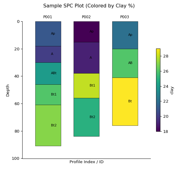
print(subset)
#> <SoilProfileCollection> (3 profiles, 12 horizons)
#>   Profile ID:   id
#>   Horizon ID:   hzid
#>   Depth Cols:   top (top), bottom (bottom)
#>   Profile Top Depths:    [min: 0.0, mean: 0.0, max: 0.0]
#>   Profile Bottom Depths: [min: 76.0, mean: 83.7, max: 91.0]
#>   Hz Desgn Col: hzname
#>   Site Vars:    id, group, elev, slope_field, aspect_field (5 total)
#>   Horizon Vars: hzid, id, hzname, genhz, top... (9 total)

ap2 = subset2.plot(color="clay", label_hz=True) # Color by clay content
import matplotlib.pyplot as plt
plt.suptitle("Sample SPC Plot (Colored by Clay %)")
plt.show()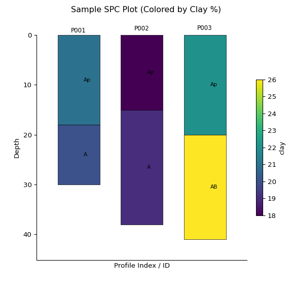
print(subset2)
#> <SoilProfileCollection> (3 profiles, 6 horizons)
#>   Profile ID:   id
#>   Horizon ID:   hzid
#>   Depth Cols:   top (top), bottom (bottom)
#>   Profile Top Depths:    [min: 0.0, mean: 0.0, max: 0.0]
#>   Profile Bottom Depths: [min: 30.0, mean: 36.3, max: 41.0]
#>   Hz Desgn Col: hzname
#>   Site Vars:    id, group, elev, slope_field, aspect_field (5 total)
#>   Horizon Vars: id, hzid, hzname, genhz, top... (9 total)

ax = x.plot(color="clay", label_hz=True) # Color by clay content
import matplotlib.pyplot as plt
plt.suptitle("Sample SPC Plot (Colored by Clay %)")
plt.show()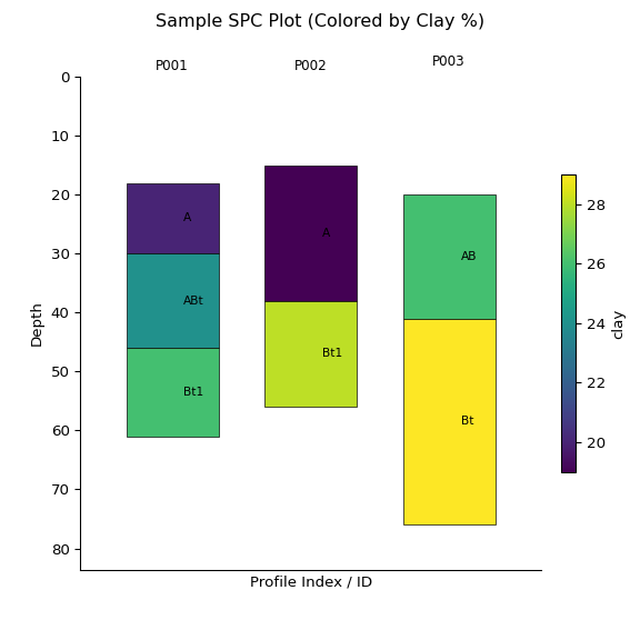
print(x)
#> <SoilProfileCollection> (3 profiles, 7 horizons)
#>   Profile ID:   id
#>   Horizon ID:   slice_hzid
#>   Depth Cols:   top (top), bottom (bottom)
#>   Profile Top Depths:    [min: 15.0, mean: 17.7, max: 20.0]
#>   Profile Bottom Depths: [min: 56.0, mean: 64.3, max: 76.0]
#>   Hz Desgn Col: hzname
#>   Site Vars:    id, group, elev, slope_field, aspect_field (5 total)
#>   Horizon Vars: hzid, id, hzname, genhz, top... (10 total)

ay = y.plot(color="clay", label_hz=True) # Color by clay content
import matplotlib.pyplot as plt
plt.suptitle("Sample SPC Plot (Colored by Clay %)")
plt.show()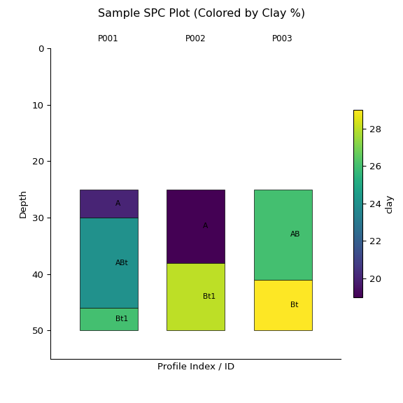
print(y)
#> <SoilProfileCollection> (3 profiles, 7 horizons)
#>   Profile ID:   id
#>   Horizon ID:   slice_hzid
#>   Depth Cols:   top (top), bottom (bottom)
#>   Profile Top Depths:    [min: 25.0, mean: 25.0, max: 25.0]
#>   Profile Bottom Depths: [min: 50.0, mean: 50.0, max: 50.0]
#>   Hz Desgn Col: hzname
#>   Site Vars:    id, group, elev, slope_field, aspect_field (5 total)
#>   Horizon Vars: hzid, id, hzname, genhz, top... (10 total)

az = z.plot(color="clay", label_hz=True) # Color by clay content
import matplotlib.pyplot as plt
plt.suptitle("Sample SPC Plot (Colored by Clay %)")
plt.show()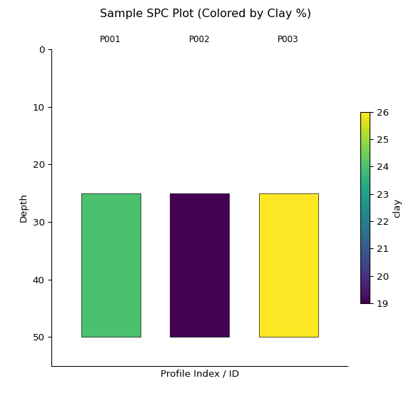
print(z)
#> <SoilProfileCollection> (3 profiles, 3 horizons)
#>   Profile ID:   id
#>   Horizon ID:   agg_hzid
#>   Depth Cols:   top (top), bottom (bottom)
#>   Profile Top Depths:    [min: 25.0, mean: 25.0, max: 25.0]
#>   Profile Bottom Depths: [min: 50.0, mean: 50.0, max: 50.0]
#>   Site Vars:    id, group, elev, slope_field, aspect_field (5 total)
#>   Horizon Vars: id, top, bottom, hzname, genhz... (9 total)