cuBNM toolbox is designed for efficient brain network modeling on GPUs.

Documentation can be found here. Read the preprint on bioRxiv.

Overview

cuBNM toolbox uses GPUs to efficiently run simulations of brain network models consisting of nodes which are connected through a connectome, and fit them to empirical neuroimaging data through integrated optimization algorithms.

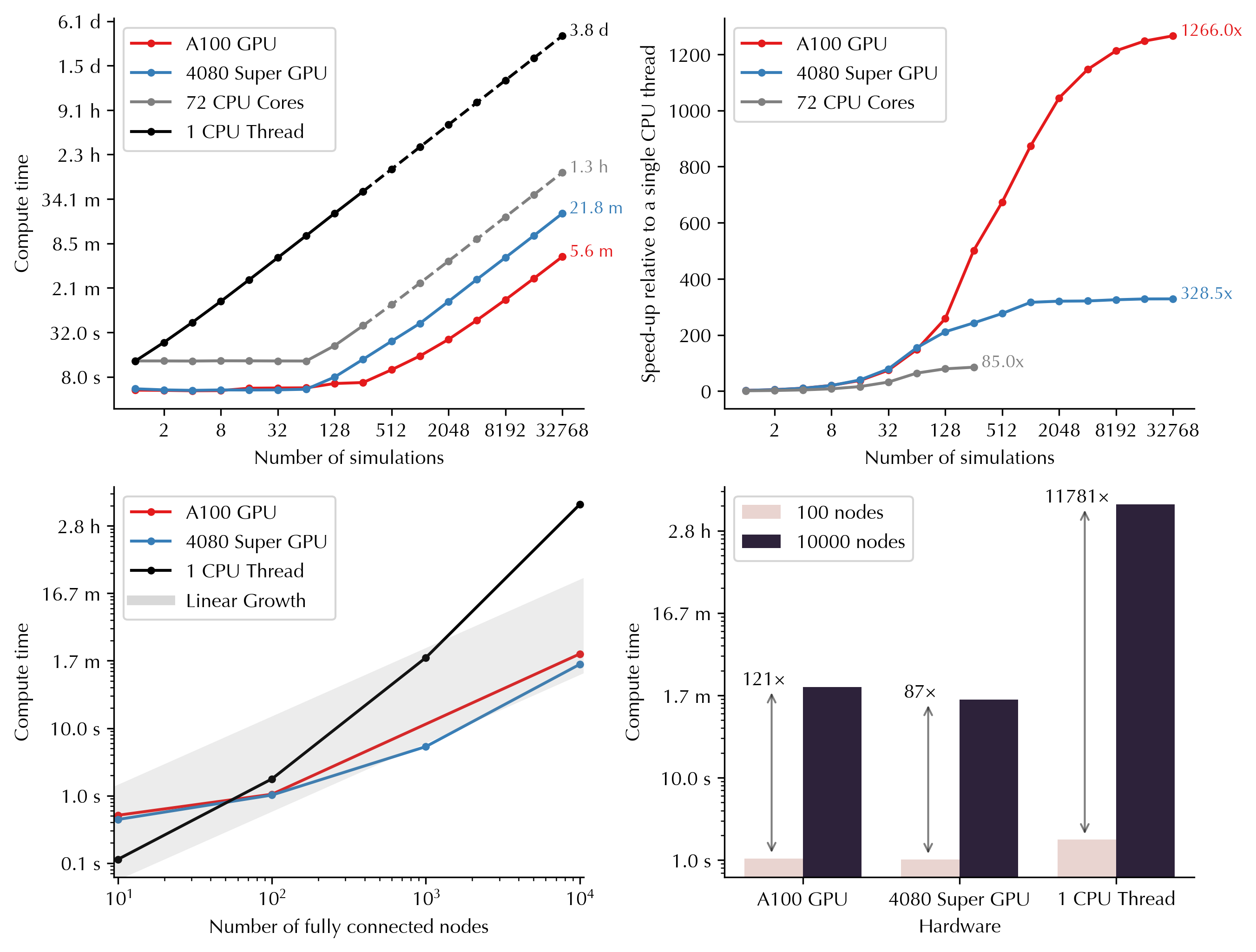
GPU parallelization enables massive scaling of the simulations into higher number of simulations and nodes. Below you can see how computing time varies as a function of number of simulations and nodes on GPUs versus CPUs. For example, running 32,768 simulations (duration: 60s, nodes: 100) would take 3.8 days on a single CPU thread, but only 5.6 minutes on Nvidia A100 GPU, and 21.8 minutes on Nvidia GeForce RTX 4080 Super:

GPU usage is the primary focus of the toolbox but it also supports running the simulations on single or multiple cores of CPU. CPUs will be used if no GPUs are detected or if requested by the user.

Several commonly used models (e.g., reduced Wong-Wang, Jansen-Rit, Kuramoto, Wilson-Cowan) are implemented, and new models can be added via YAML definition files. A guide is included on the structure of model definition YAML files to help researchers implement custom models.

The simulated activity of model neurons is fed into the Balloon-Windkessel model to calculate simulated BOLD signal. Functional connectivity (FC) and functional connectivity dynamics (FCD) from the simulated BOLD signal are calculated efficiently on GPUs/CPUs and compared to FC and FCD matrices derived from empirical BOLD signals to assess similarity (goodness-of-fit) of the simulated to empirical BOLD signal. The toolbox supports parameter optimization algorithms including grid search and evolutionary optimizers (via pymoo), such as the covariance matrix adaptation-evolution strategy (CMA-ES). Parallelization within the grid or the iterations of evolutionary optimization is done at the level of simulations (across the GPU ‘blocks’), and nodes (across each block’s ‘threads’). The models can incorporate global or regional free parameters that are fit to empirical data using the provided optimization algorithms. Regional parameters can be homogeneous or vary across nodes based on a parameterized combination of fixed maps or independent free parameters for each node or group of nodes.

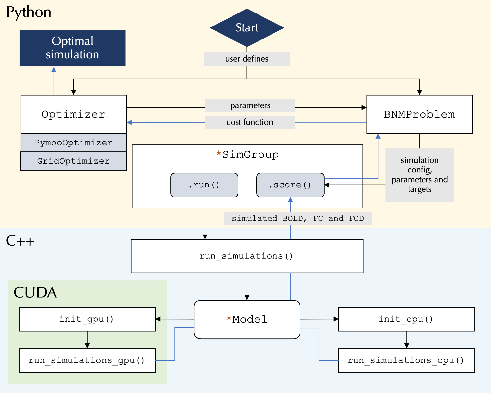
At its core the toolbox runs highly parallelized simulations using C++/CUDA, while the user interface is written in Python and allows for user control over simulation configurations:

Installation

pip install cubnm

For detailed installation instructions, including how to install from source and use Docker/Singularity containers, see the installation documentation.

System requirements

• Linux or Windows Subsystem for Linux (WSL) on x86-64 architecture
• Python >= 3.7

For GPU functionality:

• NVIDIA GPU with Compute Capability >= 6.0 (older devices with >= 2.x may work but are untested)
• NVIDIA Driver >= 520.61.05

Example usage

The following example demonstrates how to fit the rWW model to example data (included in the package) by performing a grid search over the parameters G, w_p, and J_N:

from cubnm import datasets, optimize

problem = optimize.BNMProblem(
    model = 'rWW',
    params = {
        'G': (0.001, 10.0),
        'w_p': (0, 2.0),
        'J_N': (0.001, 0.5),
    },
    duration = 60,
    TR = 1,
    window_size=10,
    window_step=2,
    sc = datasets.load_sc('strength', 'schaefer-100'),
    emp_bold = datasets.load_bold('schaefer-100'),
)
go = optimize.GridOptimizer()
go.optimize(problem, grid_shape={'G': 4, 'w_p': 5, 'J_N': 5})
go.save()

The same grid search can also be executed via the command line interface by running cubnm in the terminal:

cubnm grid \
    --model rWW --sc example --emp_bold example \
    --out_dir ./grid_cli \
    --TR 1 --duration 60 --window_size 10 --window_step 2 \
    --params G=0.001:10.0,w_p=0:2.0,J_N=0.001:0.5 \
    --grid_shape G=4,w_p=5,J_N=5 --sim_verbose

Alternatively, the model can be fitted using an evolutionary optimizer such as CMA-ES:

from cubnm import datasets, optimize

problem = optimize.BNMProblem(
    model = 'rWW',
    params = {
        'G': (0.001, 10.0),
        'w_p': (0, 2.0),
        'J_N': (0.001, 0.5),
    },
    duration = 60,
    TR = 1,
    window_size=10,
    window_step=2,
    sc = datasets.load_sc('strength', 'schaefer-100'),
    emp_bold = datasets.load_bold('schaefer-100'),
)
cmaes = optimize.CMAESOptimizer(popsize=20, n_iter=10, seed=1)
cmaes.setup_problem(problem)
cmaes.optimize()
cmaes.save()

Or via the command line interface:

cubnm optimize \
    --model rWW --sc example --emp_bold example \
    --out_dir ./cmaes_homo_cli \
    --TR 1 --duration 60 --window_size 10 --window_step 2 \
    --params G=0.001:10.0,w_p=0:2.0,J_N=0.001:0.5 \
    --optimizer CMAES --optimizer_seed 1 --n_iter 2 --popsize 10

Note: These are minimal examples intended only to demonstrate the package's basic usage and should not be used for actual research without proper configuration. For comprehensive information about brain network models and parameter fitting using grid search and evolutionary optimizers, including additional examples and detailed explanations of all features, see the tutorials.

Citation

If you use cuBNM in your work, please cite:

Saberi et al., cuBNM: GPU-Accelerated Brain Network Modeling. bioRxiv (2025) [link].

In addition, please cite the original papers for the BNMs and optimization algorithms you use.