Housing Prices Regression

Group members: Ananda Gowda, Jingqi Feng

In this project, we want to predict housing prices according to provided housing information using polynomial regression. By cleaning and encoding data set, determining the most correlated variables, and employing polynomial regression models with different degree, we find a suitable model to capture the correlation between the sale prices with the predictor variables.

Instructions of installing the package requirements: conda create --name NEWENV --file requirements.txt

Detailed description of the demo file:

1. Read the data set you're going to exam and name it "data". (In the demo file, we use the housing dataset as an example)
2. If you inspect "data", you can see there are 1460 rows and 81 columns. The dataframe consists both numerical and categorical variables.
3. Data cleaning step: import the function data_encoder to convert all categorical variables into numerical values.
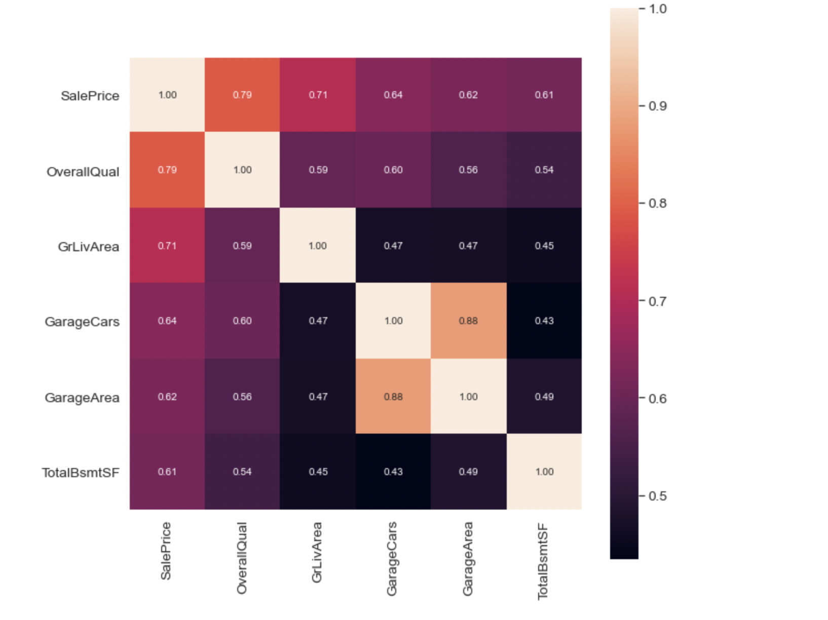
4. Use seaborn to create a correlation matrix of the 6 variables most correlated with SalePrice, and plot the correlation matrix.

In this heatmap, you can see each block contains the correlation coefficient between two specific variables. White means the correlation is very strong while black means the correlation is relatively weak. We removed "GarageArea" variable to reduce collinearity.

5. Data analyzing step: import the class Model and function PolynomialRegression.
6. If the degree is 1, this means the model is the linear regression. (In the demo file, we named it as "lr")
   • print(lr) gives some information about the linear regression model. In the demo file, you can expect to see "This is a linreg model which predicts SalePrice using the following predictors: OverallQual, GrLivArea, GarageCars, TotalBsmtSF."
   • lr.score() returns the coefficient of determination of the model on the test set. We got a score 0.6594662034635388 in the demo.
   • lr.cv_score() gives the cross-validation score with 10 splits. We got a score 0.79596462234986.
   • lr.plot() makes regression plots for each feature in predictor data.

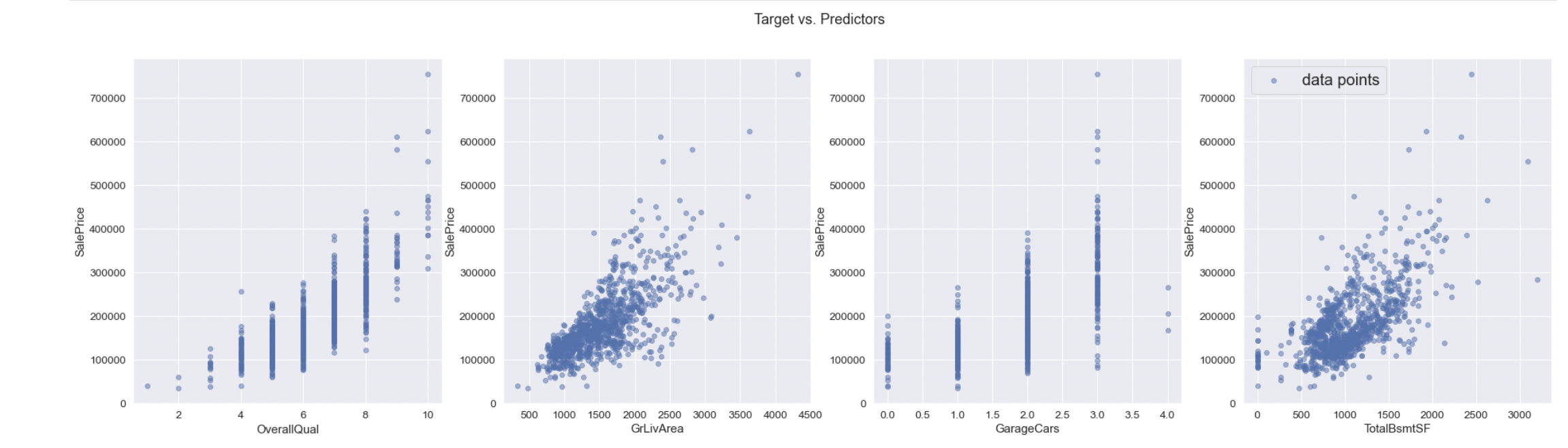
From the plots we can see there is positive correlation in for each variable with the saleprice. "OverallQual" and "GarageCars" are discrete variables so the plots contain straight lines.

7. If the degree is 2, this means the model is a ploynomial regression. (In the demo file, we named it as "pr")
   • print(pr) gives some information about the linear regression model. In the demo file, you can expect to see "This is a polyreg model which predicts SalePrice using the following predictors: OverallQual, GrLivArea, GarageCars, TotalBsmtSF."
   • pr.score() returns the coefficient of determination of the model on the test set. We got a score 0.8395161805875058 in the demo.
   • pr.cv_score() gives the cross-validation score with given number of splits. We got a score 0.7998677277567371 in the demo.
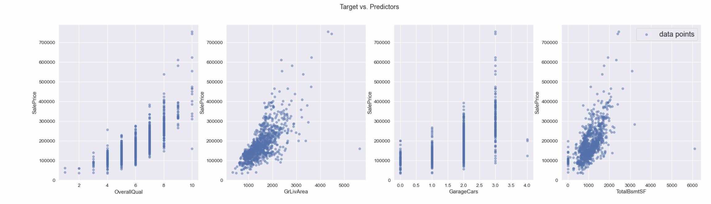
   • pr.plot() makes regression plots for each feature in predictor data.

By comparing the cross validation score from each model, the one with higher score is better to predict the housing prices. You will receive different scores for each run due to randomness. In the demo file, we can conclude that the polynomial regression with degree 2 is better since it has a higher cross-validation score.

8. Exception handling examples:
   • if the input model is not of type sklearn.pipeline.Pipeline, you can expect that a TypeError.
   • if the target variable y, which is the saleprice, does not only have one column, you can expect that a ValueError.

Scope and limitations:

1. The data collection might invade the privacy of the house owners and selling agencies, so we need to ensure that the data we're examining is appropriately collected.
2. Potential extensions: applying different regression models such as XGBoost, Ridge, and Lasso Regression.

License and terms of use See LICENSE.

References and acknowledgement Scikit-learn: https://scikit-learn.org/stable/modules/generated/sklearn.linear_model.LinearRegression.html Seaborn: https://seaborn.pydata.org/generated/seaborn.heatmap.html?highlight=heatmap#seaborn.heatmap

Data source: https://www.kaggle.com/c/house-prices-advanced-regression-techniques/data The data set contains 79 explanatory variables describing (almost) every aspect of residential homes in Ames, Iowa.