Wave-equation

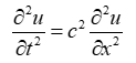
The wave equation describes the propagation of waves under ideal circumstances using the partial differential equation.

There are two second partial derivatives. One that describes time and one that describes space.

The solution is computed using 4 steps:

1. Error checking is done to ensure that 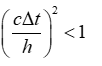. If that condition is not met, the calulated ratio as well as the acceptable nt value should be provided.
2. Initilize the matrix as well as the boundary values
3. Solving for the next column using Euler's method
4. If there are insulated boundary conditions, after the interior points of the column has been evaluated, it has to be readjusted to account for the insulated boundary conditions.

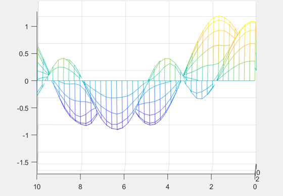
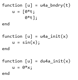
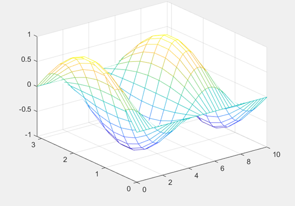
Example: Solving the wave equation using the command [x4a, t4a, U4a] = wave1d( 1, [0, pi], 10, [0, 10], 42, @u4a_init, @du4a_init, @u4a_bndry ) and displaying the solution using mesh( t4a, x4a, U4a )

Example: Solving the wave equation using the command [x4a, t4a, U4a] = wave1d( 1, [0,pi], 10, [0, 3*T], n_t, @u4a_init, @du4a_init, @u4a_bndry ) where one of the boundary conditions is insulated.

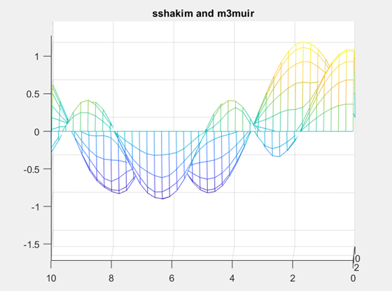
Because there is an insulated boundary at one end, when it gets to that end, the wave will travel in a reflected direction rather than going back in the same direction. The period in both direction is the same however they are shifted due to the insulated boundary.