CNN-without-Keras

I implement a convolutional neural network (CNN) architecture using a deep learning library. The best way to learn how a system works, you need to build it from scratch, hence you will be able to see the problems you may encounter and find the solutions to them or how to improve your model in next phases. Therefore; I did not use off-the-shelf architectures, e.g., VGG. I use CIFAR10 dataset. I implement my network in Tensorflow. I did not use preset functions to compile my model or get predictions (e.g., model.compile, model.predict functions in Keras).

How to Run

File Folder Format

• cifar10_data
  • cifar10_data
    data_batch_1
    data_batch_2
    data_batch_3
    data_batch_4
    data_batch_5
    test_batch
    
  • model.py
• main.py
• eval.py
• Execute "python main.py" to run model with the final hyperparameters and optimizer. I set epoch number to 100. I dumped model at some epoches (at the beginning, at the middle and at the end of training) You can update it in the code.
• "python eval.py" to see test accuracy of fully trained model. I commented out t-sne plotting section since it takes too much time.

Data Augmentation

I used various augmentation techniques which are random flip, random rotate, random color change and random zooming (includes cropping) (a). I applied these techniques in different combinations to randomly chosen data samples from training set. At the end, I have 24,000 generated images with augmentation techniques and 74,000 images in total for training and validation. The function ’prepare cifar10’ in model.py can be analyized for further information.

Network Architecture and Improvements

I designed a 3-layer CNN architecture for object classification task. Since a 3-layer CNN did not give me the state-of-the-art performance on CIFAR10 data. I explored ways to obtain as high performance as possible with the 3-layer CNN.

• Reasoning behind my choices on the kernel size, activation functions, number of feature maps, number of fully connected layers, and the size of the fully connected layers.

  • First of all, I set learning rate to 0.004, chose AdaGrad as optimizer and set batch size to two to the power of nine (512). Smaller batch sizes increase computation time as well as accuracy which means there is a trade off. I will decrease batch size in following steps and come to a decision. Additionally, I run the model for 20 epoches at first iterations since I run many models and it would be costly in time to run them for more epoches.
  • As to kernel size decision, I should state the impact of kernel size first. If we use larger kernel size; computational time will be faster, memory usage will be smaller; however, we will lose lot of details. For example, let’s say we have NxN input neuron and the kernel size is NxN too, then the next layer only gives use one neuron. Loss lot of details can cause underfitting. On the other hand, smaller kernel will give us lot of details. Our image sizes are 32 x 32 (relatively small) so I decided to use small kernel size (3x3) to keep details of image.
  • As to activation function, I used Relu. In data preperation, we already normalized our input data so we will not likely to encounter exploding gradient problem. On the other hand, it is easier to compute since the mathematical function is easier and simple than other activation functions. Since we work with image data, I put emphasize on computational time and memory usage. Additionally, I did some research and realize that Relu is best-practice for this case.
  • As going deeper through convolution layers, number of feature maps increases with power of 2 whereas width x height decreases by pooling. I tried to extract as many features as I can through layers. I built models with different number of feature maps to analyze accuracy and loss. It does not mean increasing feature map number will result in better performance. After some point, it may detect some other parts apart from our desired object and the activations die out at a certain layer and computational burden increases by increasing number of feature maps. For example, I plotted accuracy and loss of 20 epochs for two different models and stated them in Figure 1.

  

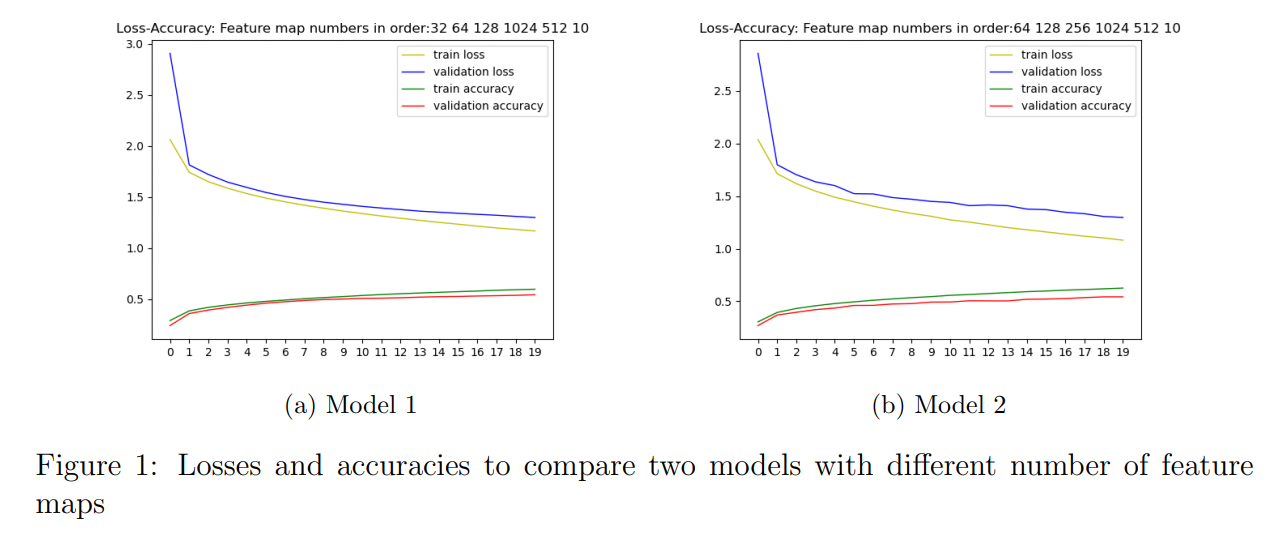
  • As can be seen from Figure 1, increasing feature map number from Model 1 to Model 2 did not increase performance of model that much but added computational work. So I chose Model 1 at this point. Additionally, I used 1 stride not to lose information in convolution layers.
  • As to fully connected layers, I used two of them after flatted the output of CNN. Most important part is I want the fully connected layer just has enough number of neurons so as to capture variability of the entire input. Therefore, I put two fully connected layers which sizes decrease gradually.
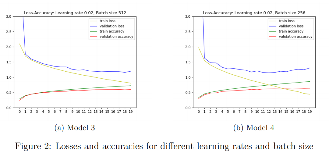
  • Then, I increased learning rate to 0.02 and decreased batch size to 256 step by step. I plotted losses and accuracies respectively and show them in Figure 2. Increasing learning rate to 0.02 resulted in decrease in training and validation loss and increase in training and validation accuracy (compared Model 1 and Model 3). Decreasing batch size to 256 resulted in increase in training and validation accuracy but approximately no change in validation loss (compared Model 3 and Model 4).

  

• Techniques to improve the performance, such as adding dropout, batch normalization, residual blocks. My observations on the effect of these techniques on the performance.

  • After second step, I used batch normalization before Relu in convolution layers to standardize layer inputs. I did research and saw that batch normalization eliminates the need for dropout in some cases cause batch normalization provides similar regularization benefits as dropout intuitively (b). Therefore I do not use dropout since I used batch normalization and I did not have overfitting problem. Additionally, dropout added more computation because of additional matrices for dropout masks, drawing random numbers for each entry of these matrices and multiplying the masks and corresponding weights. At this step, I increased the epoch number to 100 and set an early stopping condition based on calculated loss during training. I explain it in detail in the following question. I plotted the accuracy and loss for regarding epoch number and show it in Figure 3.

  

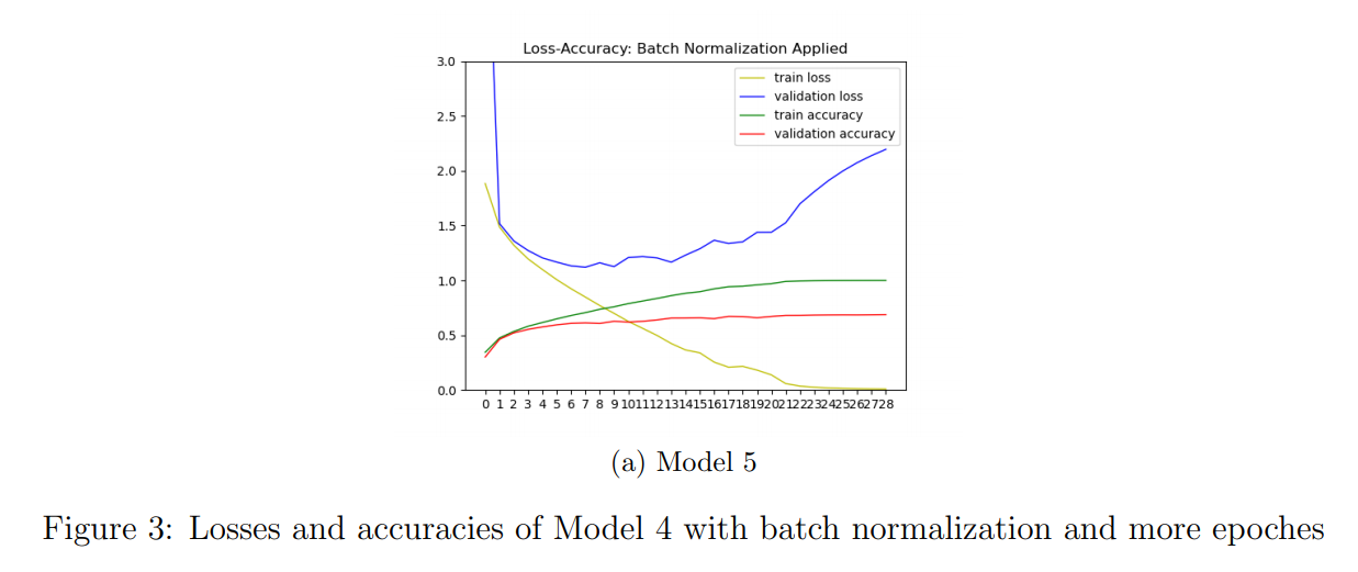
  • As can be seen from Model 5 in Figure 3, validation and training accuracies increased whereas training loss decreased. I wanted to point out that validation accuracy increased from first epoches to last ones. That is, it increased in first 20 epoches in Model 5 compared to Model 4.
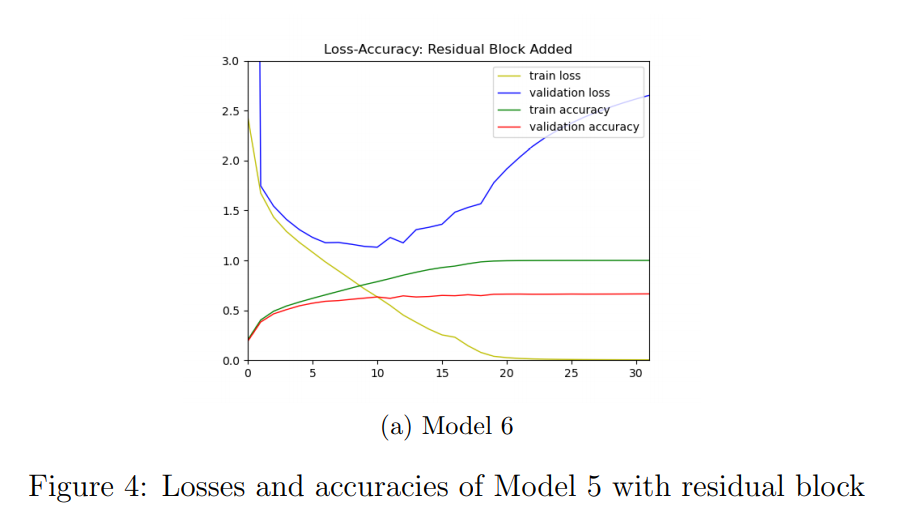
  • I also added residual block at the end of convolution layers. I analyized its effect on accuracy and loss. Plotted these metrics with respect to the epoches which is showed in Figure 4 and see that there is no improvement.

  

• Choosing an optimizer and training my network. The value of the loss function with respect to number of epochs. Decision of the batch size. Training and test classification accuracy. Early stopping procedure.

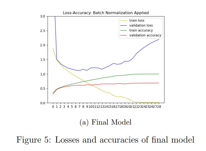
  • I chose AdaGrad as optimizer firstly. I plotted final model loss function values with respect to number of epochs determined by stopping condition which is stated it in Figure 5. Test accuracy of the final model is 0.7208. Validation accuracy of last epoch of the final model is 0.6925. Training accuracy of last batch of last epoch of the final model is 0.6925.

  

  • I stated the reason for choosing batch size 256 (two to the power of eight) step by step in previous sections. The behaviour of the my early stopping condition depends on three factors: validation loss (metric), an improvement between the performance of the monitored loss in the current epoch and the best result in that metric, and the number of epochs without improvements before stopping. I calculated average validation loss per epoch. At the end of each epoch, I check if current average validation loss is higher of lower than lowest (best) validation loss and updated lowest (best) validation loss. If there is no improvement in validation loss for 20 epoch, then I stopped training the model.

• Trying different optimizers and comparing their performance and convergence properties.

  • I used AdaGrad optimizer in final model. Then, I tried other optimizers. Results with Gradient Descent Optimizer is as following in Figure 6.

  

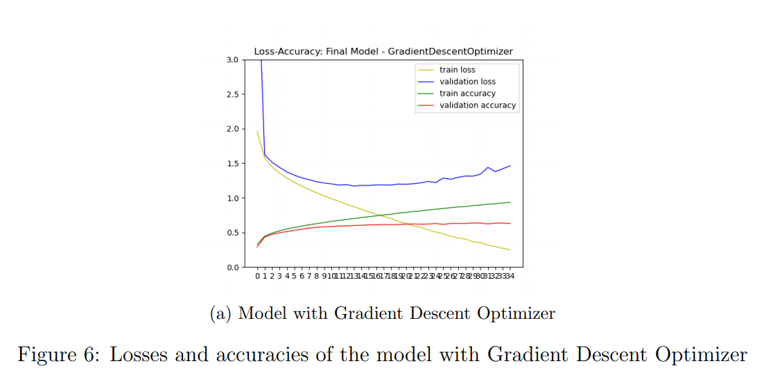
  • Test accuracy of the model with Gradient Descent Optimizer is 0.6854. Results with RMSProp Optimizer is as following in Figure 7.

  

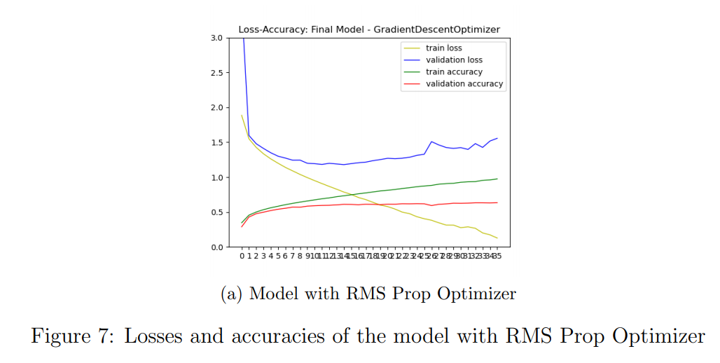
  • Test accuracy of the model with RMS Prop Optimizer 0.6778.
  • Gradient Descent Optimizer is simplest version of optimizers I used. I just updates parameters just by subtructing multiplication of learning rate and gradient from them. AdaGrad decays the learning rate for parameters in proportion to their update history. However AdaGrad decays the learning rate very aggressively (as the denominator grows). After a while, the parameters start receiving very small updates because of the decayed learning rate. To avoid this RMS Prop decays the denominator and prevents its rapid growth. I observed that Ada Grad is better in training loss (additionally in validation accuracy) compared to RMS Prop. It means we need to decay learning rate aggressively through training. I chose go with the AdaGrad optimizer.

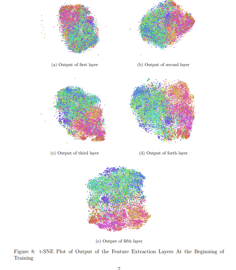
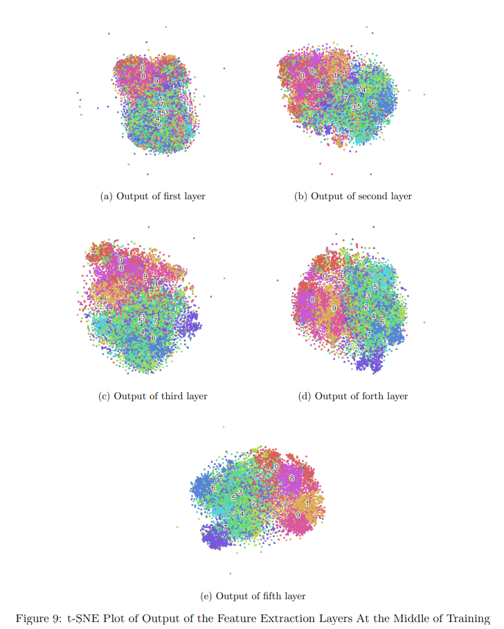
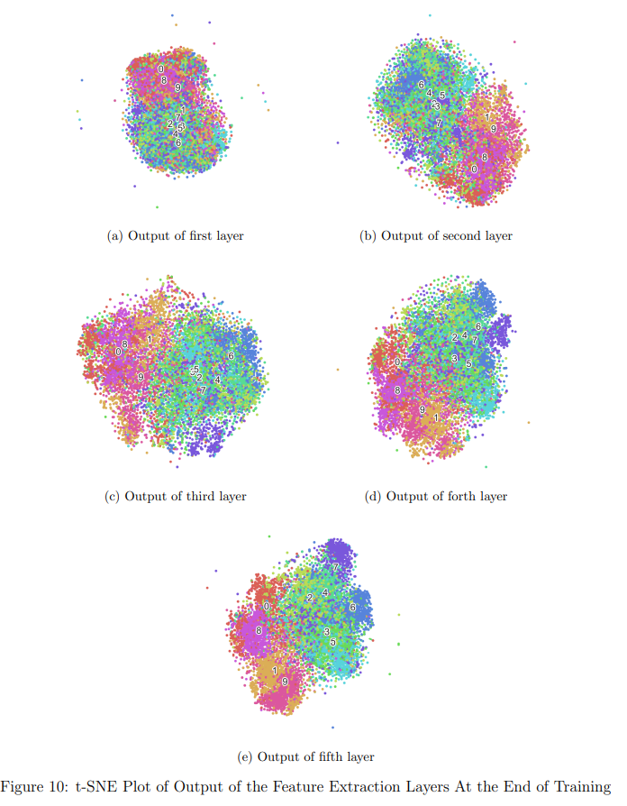
• Visualizing the latent space of the model for the training samples (output of the feature extraction layers) in the beginning of the training, in the middle of the training, and in the end of the training.

  • To visualize, I map the latent representations into 2-D space using t-SNE. Different colors are used to illustrate the categories.
  • We can see below that groups are separated and centered at different points via intensified colors at these points at the end of the training.