Sec. I. Introduction and Overview
Sec. II. Theoretical Background
Sec. III. Algorithm Implementation and Development
Sec. IV. Computational Results
Sec. V. Summary and Conclusions
The MNIST dataset is a well-known dataset of handwritten digits that is often used in machine learning research. In this project, the goal is to perform an analysis of the MNIST dataset, including an SVD analysis of the digit images, building classifiers to identify individual digits in the training set, and comparing the performance of LDA, SVM, and decision tree classifiers on the hardest and easiest pair of digits to separate.
The MNIST dataset is a large collection of handwritten digit images that has become a standard benchmark for testing machine learning algorithms. In this analysis, we will perform an in-depth analysis of the MNIST dataset, including an SVD analysis of the digit images, building a classifier to identify individual digits in the training set, and comparing the performance of different classification algorithms.
We will start by performing an SVD analysis of the digit images, which involves reshaping each image into a column vector and using each column of the data matrix as a different image. We will analyze the singular value spectrum and determine how many modes are necessary for good image reconstruction (i.e. the rank r of the digit space). We will also interpret the U, Σ, and V matrices in this context.
Next, we will project the data into PCA space and build a classifier to identify individual digits in the training set. We will start by picking two digits and building a linear classifier (LDA) that can reasonably identify/classify them. Then we will pick three digits and try to build a linear classifier to identify these three. We will determine which two digits in the data set appear to be the most difficult to separate and quantify the accuracy of the separation with LDA on the test data. We will also determine which two digits in the data set are most easy to separate and quantify the accuracy of the separation with LDA on the test data.
Finally, we will compare the performance between LDA, SVM, and decision trees on the hardest and easiest pair of digits to separate (as determined in the previous step). SVM and decision tree classifiers were the state-of-the-art classification techniques until about 2014, and we will see how well they separate between all ten digits in the MNIST dataset.
The MNIST dataset is a popular dataset for image classification and machine learning tasks. It consists of 70,000 handwritten digits, with 60,000 images in the training set and 10,000 images in the test set. Each image is a grayscale 28x28 pixel image, representing a digit from 0 to 9.
PCA (Principal Component Analysis) is a technique used to reduce the dimensionality of data while preserving the most important information in the data. It finds the principal components by performing a linear transformation of the data into a new coordinate system, where the axes are orthogonal (perpendicular) and ranked by the amount of variance they explain in the data. The first principal component is the direction of maximum variance, the second principal component is the direction of maximum variance that is orthogonal to the first, and so on.
Mathematically, PCA finds the principal components by computing the eigenvectors and eigenvalues of the covariance matrix of the data. The eigenvectors represent the directions of the principal components, while the eigenvalues represent the amount of variance explained by each principal component. The eigenvectors are sorted by their corresponding eigenvalues in descending order, so the first eigenvector corresponds to the first principal component.
PCA can be used for various purposes such as data compression, data visualization, and feature extraction. In the context of image analysis, PCA can be used to identify the most significant features in images, and to project images onto a lower-dimensional space for further analysis or visualization.
SVD (Singular Value Decomposition) is a more general decomposition method that can be applied to any matrix, unlike eigendecomposition, which is only applicable to square matrices. In this project, we will use SVD to visualize the singular value spectrum and use this to find the rank r of the digit space.
SVD is a matrix factorization technique that decomposes a matrix M (mn) into three matrices: U, Σ, and V (in the code, these matricies have respectively been called U, s, and V). The matrix Σ is diagonal and contains the singular values (in decreasing order) of the original matrix, which correspond to the square roots of the eigenvalues of the covariance matrix of the data. The matrix U contains the left singular vectors, and the matrix V* contains the right singular vectors.
It is important to note that any time a matrix A is multiplied by another matrix B, only two primary things can occur: B will stretch and rotate A. Hence, the three matricies SVD splits a matrix M into simply rotate M (V*), stretch M (Σ), and rotate M (U).
This concept can be visualized in figure 1 below. If we have a 2D disk (of a real sqaure matrix M), rotation first occurs, then stretching M will create an elipse with major and minor axes σ1 and σ2, and then we rotate again and find ourselves in a new coordiante system. We can say that u1 and u2 are unit orthonormal vectors known as principal axes along σ1 and σ2 and σ1 and σ2 are singular values. Thus, u1 and u2 determine the direction in which the stretching occurs while the singular valeus determine the magnitude of this stretch (eg. σ1u1).
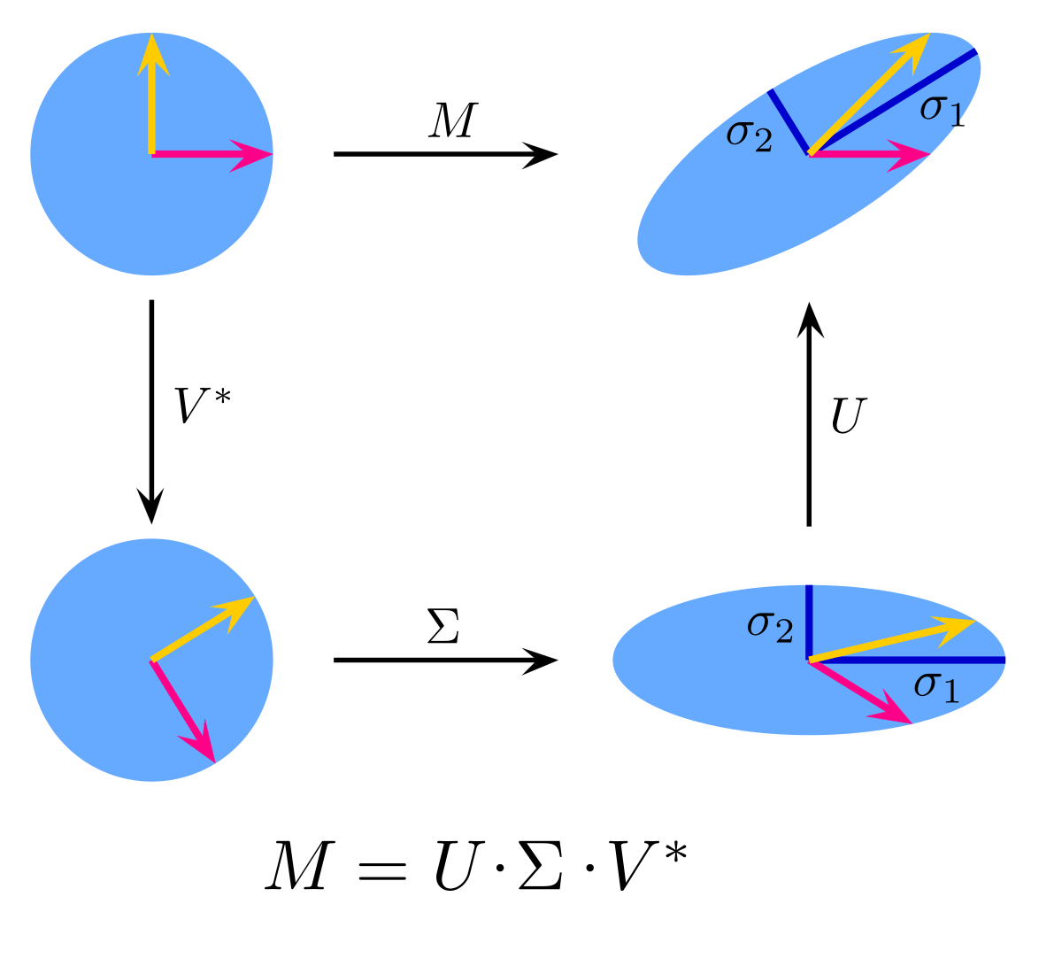 Figure 1: Visualization of the 3 SVD matrices U, Σ, and V
In the context of PCA, the principal components can be obtained from the right singular vectors of the data matrix. This is because the right singular vectors are the eigenvectors of the covariance matrix of the data. Therefore, the right singular vectors are often called the PCA modes.
However, the left singular vectors of the data matrix can also be useful in some applications, such as in image compression. In this case, the left singular vectors are called the SVD modes. The SVD modes and the PCA modes are related, but they are not exactly the same thing, as the SVD modes are not guaranteed to be orthogonal, while the PCA modes are always orthogonal.
LDA (Linear Discriminant Analysis), SVM (Support Vector Machines), and decision tree classifiers are machine learning algorithms used for classification tasks.
LDA (Linear Discriminant Analysis) is a linear classification method that finds a linear combination of features that best separates the classes in the data. It assumes that the data is normally distributed, and the classes have the same covariance matrix. LDA can be used for binary and multiclass classification tasks.
SVM (Support Vector Machines) is a non-linear classification method that finds a hyperplane that separates the classes in the data with the largest margin. It uses a kernel function to map the data into a higher-dimensional space, where the classes are linearly separable. SVM can be used for binary and multiclass classification tasks, and is known for its ability to handle high-dimensional data.
Decision tree classifiers are a type of algorithm that uses a tree-like model of decisions and their possible consequences to classify the data. It works by splitting the data into subsets based on the values of one feature at a time, until the subsets are as pure as possible (i.e., they only contain data points from one class). The tree structure can be used to interpret the classification decisions made by the algorithm.
All three classifiers have their own advantages and disadvantages, and their performance can vary depending on the specific data and task at hand. LDA and SVM are commonly used for classification tasks in a wide range of fields, while decision trees are often used in applications where interpretability is important.
Firstly, I loaded the MNIST dataset from the scikit-learn library using the fetch_openml function:
from sklearn.datasets import fetch_openml

# Load the MNIST dataset
mnist = fetch_openml('mnist_784')

# Reshape each image into a column vector
X = mnist.data.T / 255.0  # Scale the data to [0, 1]
Y = mnist.target.astype('int32')
The MNIST dataset is a 2D array where each row corresponds to an image and each column corresponds to a pixel value. This code uses the transpose (.T) method to convert the dataset into a 784x70000 array where each column corresponds to an image and each row corresponds to a pixel value. This is often a more convenient format for performing computations and analyses.
Additionally, the pixel values are divided by 255 to scale them down to a range of [0,1]. This is because the original pixel values range from 0-255, but many machine learning algorithms work better when the data is scaled to be between 0 and 1.
Also, this code creates an array Y containing the target labels for each image in the dataset. These labels indicate which digit (0-9) is shown in each image, and will be used as the target variable for classification tasks.
We then run SVD and store the three matricies formed in variables U, s, and V:
# Perform SVD on X
U, s, V = np.linalg.svd(X, full_matrices=False)
As discussed in the theoretical background section, we can use the s (Σ) matrix to obtain the singular values in descending order. Hence, we can simply plot s to get the singular value spectrum like this:
# Plot the singular value spectrum
plt.plot(s)
plt.xlabel('Singular Value Index')
plt.ylabel('Singular Value')
plt.show()
The singular value spectrum from SVD represents the singular values of the original matrix. In the context of image reconstruction, it represents the amount of energy captured by each mode (or singular value) of the SVD. The singular values are arranged in decreasing order, so the first singular value captures the most energy and the last singular value captures the least.
To determine the number of modes necessary for good image reconstruction, we need to look at the amount of energy captured by each mode. One way to do this is to calculate the cumulative sum of the singular values and normalize by the total sum of all singular values. Then we can plot this cumulative sum and look for an "elbow" or "knee" point where adding more modes does not contribute much to the total energy captured.
The rank r of the digit space can be determined by looking at the number of non-zero singular values in the singular value spectrum. This is because the rank of the original matrix is equal to the number of non-zero singular values. We use the following snippet of code to plot the cumulative sum and then find r:
# Plot the cumulative sum of the singular values
plt.plot(np.cumsum(s)/np.sum(s))
plt.xlabel('Singular Value Index')
plt.ylabel('Cumulative Sum')
plt.show()

# Set the threshold for the amount of variance to retain
threshold = 0.46

# Calculate the number of dimensions to keep
k = np.argmax(np.cumsum(s) >= threshold*np.sum(s)) + 1

# Calculate the number of singular values greater than s[k-1] (where k is the number of dimensions to keep)
r = np.sum(s > s[k-1])

# Print the number of dimensions and the number of retained singular values
print('k:', k)
print('r:', r)
Here, the code first sets a threshold for the amount of variance to retain from the SVD, which is a value between 0 and 1. It then uses the cumulative sum of the singular values (stored in s) to find the index (k) of the last singular value that, when added to the sum of the preceding singular values, exceeds the threshold times the total sum of the singular values. The number of dimensions to keep is then k. Finally, the number of singular values greater than s[k-1] is counted to obtain the number of singular values that are retained, which is stored in r.
For a clearer view on when these singular values started to dip, I also plotted using a scree plot:
# calculate the cumulative sum of the squared singular values
cumulative_sum = np.cumsum(s**2)

# calculate the percentage of total variance captured by each singular value
variance_explained = cumulative_sum / np.sum(s**2)

# plot the scree plot
plt.plot(np.arange(1, len(s)+1), variance_explained, 'ro-', linewidth=2)
plt.axvline(x=10, color='b', linestyle='--')
plt.title('Scree Plot')
plt.xlabel('Principal Component')
plt.ylabel('Variance Explained')
plt.show()
Then, the data was projected onto different V-modes, starting with 2,3, and 5:
# Select the V-modes to use
v_modes = [2, 3, 5]

# Project the data onto the selected V-modes
X_projected = V[:, v_modes].T @ X.values

# Create a 3D plot with a larger size
fig = plt.figure(figsize=(10, 10))
ax = fig.add_subplot(111, projection='3d')

# Scatter plot the projected data with a legend
scatter = ax.scatter(X_projected[0, :], X_projected[1, :], X_projected[2, :], c=Y.astype(int), cmap='jet')
legend = ax.legend(*scatter.legend_elements(), title='Classes', loc='upper left')
ax.add_artist(legend)

# Add axis labels
ax.set_xlabel(f'V-mode {v_modes[0]}')
ax.set_ylabel(f'V-mode {v_modes[1]}')
ax.set_zlabel(f'V-mode {v_modes[2]}')

ax.set_title('Projection onto V-modes 2, 3, and 5')

# # Set the view angle
# ax.view_init(90, 0)

# Show the plot
plt.tight_layout()
plt.show()
First, we select the three V-modes (columns of the V matrix) that we want to use for the projection. Next, we compute the projection of the data matrix X onto the selected V-modes, by multiplying the transpose of the selected V-modes with the data matrix. Note that we first transpose the selected V-modes so that they have the same shape as the data matrix. The rest simply plots the data into as a scatter plot. It should be noted here that the parameter c in the scatter function represents the color of the markers in the scatter plot. It can take an array of values to color each marker differently based on some categorical or continuous variable. In this case, Y.astype(int) is passed as the argument for c, which is an array of the target values of the MNIST dataset, converted to integers. Therefore, each marker in the scatter plot will be colored based on its corresponding digit label. The cmap parameter is used to specify the colormap to use for coloring the markers. 'jet' is a popular choice of colormap that maps low values to blue, intermediate values to green and high values to red.
Now, LDA was performed to classify between 2 digits:
# LDA for 2 digits

# Transpose the data X for easier filtering using Boolean logic
Xt = X.T

# Perform PCA on the original dataset to reduce dimensionality to 10 components
pca = PCA(n_components=10)
pca.fit(Xt)
X_pca = pca.transform(Xt)

# Select only 4s and 9s in the new PCA space
X_pca_49 = X_pca[(Y == 4) | (Y == 9)]
Y_pca_49 = Y[(Y == 4) | (Y == 9)]

# Split into training and testing sets
X_pca_train, X_pca_test, Y_pca_train, Y_pca_test = train_test_split(X_pca_49, Y_pca_49, test_size=0.2, random_state=42)

# Train an LDA model on the training set using the transformed data
lda_pca = LinearDiscriminantAnalysis()
lda_pca.fit(X_pca_train, Y_pca_train)

# Make predictions on the testing set
Y_pca_pred = lda_pca.predict(X_pca_test)

# Evaluate the accuracy of the classifier
accuracy_LDA2_pca = accuracy_score(Y_pca_test, Y_pca_pred)
print(f"Accuracy: {accuracy_LDA2_pca:.2f}")
The code performs principal component analysis (PCA) on the original dataset X, with the aim of reducing the dimensionality of the dataset from the original number of features to just 10. The PCA() function is used to create a PCA object, and n_components=10 is set to specify that we want to keep only the top 10 principal components. The .fit() method is then called on the PCA object with X as input to train the PCA model, and the .transform() method is called to transform X into a new dataset X_pca with only 10 dimensions.
We filter the dataset X_pca to only include samples that correspond to the digit 4 or the digit 9, and the corresponding labels Y_pca are also filtered accordingly. The filtered dataset and labels are then split into training and testing sets using the train_test_split() function from the sklearn.model_selection module. The test_size parameter is set to 0.2 to specify that we want to use 20% of the data for testing, and random_state is set to 42 to ensure reproducibility.
A linear discriminant analysis (LDA) model is then trained on the training set using the transformed dataset X_pca_train and corresponding labels Y_pca_train. The LinearDiscriminantAnalysis() function from the sklearn.discriminant_analysis module is used to create the LDA object, and the .fit() method is called to train the LDA model. The trained LDA model is used to make predictions on the testing set X_pca_test, and the predicted labels are stored in Y_pca_pred.
Finally, the accuracy of the classifier is evaluated by comparing the predicted labels Y_pca_pred with the true labels Y_pca_test, and computing the accuracy using the accuracy_score() function from the sklearn.metrics module. The resulting accuracy is printed to the console.
The same was then done for the comparison and classification of three digits, 0, 8, and 9. The approach is entirely similar except now we must filter out the 0s, 8s, and 9s into the dataset under study:
# LDA for 3 digits
# Select only 0s and 8s and 9s
X_089 = X_pca[(Y == 0) | (Y == 8) | (Y == 9)]
Y_089 = Y[(Y == 0) | (Y == 8) | (Y == 9)]
After that, I looped through all possible combinations of digits and calculated the accuracy for all 45 unique combinations:
from itertools import combinations

# Define the list of digits to use
digits = [0, 1, 2, 3, 4, 5, 6, 7, 8, 9]

# Initialize a list to store the accuracies and corresponding digit pairs
results = []

# Loop over all pairs of digits
for digit1, digit2 in combinations(digits, 2):

    # Select the data for the current pair of digits
    X_pair = X_pca[(Y == digit1) | (Y == digit2)]
    Y_pair = Y[(Y == digit1) | (Y == digit2)]

    # Split into training and testing sets
    X_train, X_test, Y_train, Y_test = train_test_split(X_pair, Y_pair, test_size=0.2, random_state=42)

    # Train an LDA model
    lda = LinearDiscriminantAnalysis()
    lda.fit(X_train, Y_train)

    # Make predictions on the testing set
    Y_pred = lda.predict(X_test)

    # Evaluate the accuracy of the classifier
    accuracy = accuracy_score(Y_test, Y_pred)

    # Append the digit pair and accuracy to the results list
    results.append((digit1, digit2, accuracy))
The approach is the same as the two digits version execept we loop through different combinations of digits and store the pair and their accuracy in a results array. I then sorted this results array by accuracy and printed the sorted array:
# sort the results
sorted_results = sorted(results, key=lambda x: x[2], reverse=True)
# Print the sorted list of results
for result in sorted_results:
    print(f"Digits: ({result[0]}, {result[1]})\tAccuracy: {result[2]:.2f}")
The dataset was then tested for accuracy when using SVM and decision tree classifiers. The approach is the same as before except rather than fitting our data to LDA, we fit to SVC (SVM) and DecisionTreeClassifier (DTC):
#Split the data into training and testing sets
X_train_SVM, X_test_SVM, y_train_SVM, y_test_SVM = train_test_split(X_pca, Y, test_size=0.2, random_state=42)

#Scale the data using a standard scaler
scaler = StandardScaler()
X_train_SVM = scaler.fit_transform(X_train_SVM)
X_test_SVM = scaler.transform(X_test_SVM)

#Initialize an SVM classifier
svm = SVC(kernel='rbf', C=1, gamma='auto')

# Train the classifier on the training set
svm.fit(X_train_SVM, y_train_SVM)

# Make predictions on the testing set
y_pred_SVM = svm.predict(X_test_SVM)

# Evaluate the accuracy of the classifier
accuracy = accuracy_score(y_test_SVM, y_pred_SVM)
print(f"Accuracy: {accuracy:.2f}")
# Split the data into training and testing sets
X_train_DTC, X_test_DTC, y_train_DTC, y_test_DTC = train_test_split(X_pca, Y, test_size=0.2, random_state=42)

# Train a decision tree classifier with default hyperparameters
clf = DecisionTreeClassifier()
clf.fit(X_train_DTC, y_train_DTC)

# Make predictions on the testing set
y_pred_DTC = clf.predict(X_test_DTC)

# Evaluate the accuracy of the classifier
accuracy_DTC = accuracy_score(y_test_DTC, y_pred_DTC)
print(f"Accuracy: {accuracy:.2f}")
I then printed this decision tree using the plot_tree function:
# Plot the decision tree
plt.figure(figsize=(20, 10))
plot_tree(clf, filled=True)
plt.show()
The filled parameter was set to true since that fils the decision tree nodes with color for better visuilization of the classification.
Finally, the accuracy of classification of the least and most common pairs of digits (according to LDA) was compared to the accuracy when using SVM and CLF:
# Hardest pair: (4,9)
# Easiest pair: (1,0)
# Select only 4s and 9s
X_49 = X_pca[(Y == 4) | (Y == 9)]
Y_49 = Y[(Y == 4) | (Y == 9)]

# Split the data into training and testing sets
X_train_SVM_49, X_test_SVM_49, y_train_SVM_49, y_test_SVM_49 = train_test_split(X_49, Y_49, test_size=0.2, random_state=42)

# Scale the data using a standard scaler
scaler_49 = StandardScaler()
X_train_SVM_49 = scaler_49.fit_transform(X_train_SVM_49)
X_test_SVM_49 = scaler_49.transform(X_test_SVM_49)

# Initialize an SVM classifier
svm_49 = SVC(kernel='rbf', C=1, gamma='auto')

# Train the classifier on the training set
svm_49.fit(X_train_SVM_49, y_train_SVM_49)

# Make predictions on the testing set
y_pred_SVM_49 = svm_49.predict(X_test_SVM_49)

# Evaluate the accuracy of the classifier
accuracy_SVM_49 = accuracy_score(y_test_SVM_49, y_pred_SVM_49)
print(f"Accuracy: {accuracy_SVM_49:.2f}")
# Split the data into training and testing sets
X_train_DTC_49, X_test_DTC_49, y_train_DTC_49, y_test_DTC_49 = train_test_split(X_49, Y_49, test_size=0.2, random_state=42)

# Train a decision tree classifier with default hyperparameters
clf_49 = DecisionTreeClassifier()
clf_49.fit(X_train_DTC_49, y_train_DTC_49)

# Make predictions on the testing set
y_pred_DTC_49 = clf.predict(X_test_DTC_49)

# Evaluate the accuracy of the classifier
accuracy_DTC_49 = accuracy_score(y_test_DTC_49, y_pred_DTC_49)
print(f"Accuracy: {accuracy_DTC_49:.2f}")
X_10 = X_pca[(Y == 1) | (Y == 0)]
Y_10 = Y[(Y == 1) | (Y == 0)]

# Split the data into training and testing sets
X_train_SVM_10, X_test_SVM_10, y_train_SVM_10, y_test_SVM_10 = train_test_split(X_10, Y_10, test_size=0.2, random_state=42)

# Scale the data using a standard scaler
scaler_10 = StandardScaler()
X_train_SVM_10 = scaler_10.fit_transform(X_train_SVM_10)
X_test_SVM_10 = scaler_10.transform(X_test_SVM_10)

# Initialize an SVM classifier
svm_10 = SVC(kernel='rbf', C=1, gamma='auto')

# Train the classifier on the training set
svm_10.fit(X_train_SVM_10, y_train_SVM_10)

# Make predictions on the testing set
y_pred_SVM_10 = svm_10.predict(X_test_SVM_10)

# Evaluate the accuracy of the classifier
accuracy_SVM_10 = accuracy_score(y_test_SVM_10, y_pred_SVM_10)
print(f"Accuracy: {accuracy_SVM_10:.2f}")
# Split the data into training and testing sets
X_train_DTC_10, X_test_DTC_10, y_train_DTC_10, y_test_DTC_10 = train_test_split(X_10, Y_10, test_size=0.2, random_state=42)

# Train a decision tree classifier with default hyperparameters
clf_10 = DecisionTreeClassifier()
clf_10.fit(X_train_DTC_10, y_train_DTC_10)

# Make predictions on the testing set
y_pred_DTC_10 = clf.predict(X_test_DTC_10)

# Evaluate the accuracy of the classifier
accuracy_DTC_10 = accuracy_score(y_test_DTC_10, y_pred_DTC_10)
print(f"Accuracy: {accuracy_DTC_10:.2f}")
The only difference in these cases versus the previously described cases is that we must filter different values from our main PCA space dataset.
The results will be analyzed in depth in Section IV.
After running SVD, the singular values and the cumulative sum of the singular values were plotted against the singular value index:
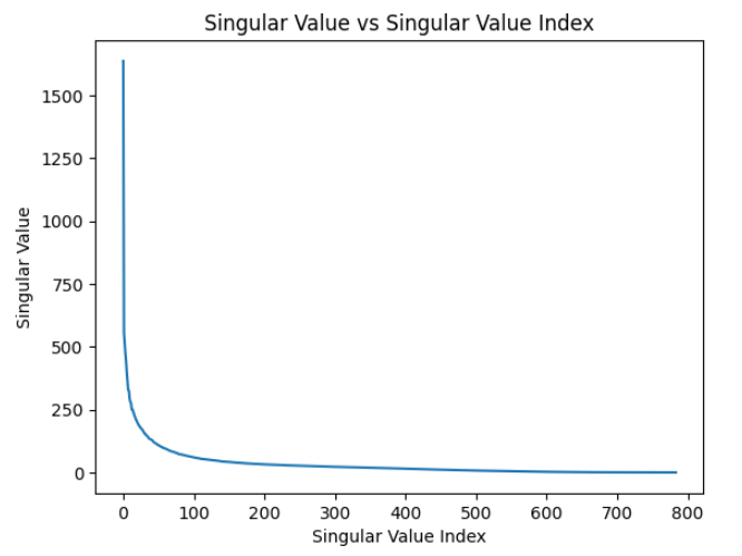 Figure 2: Singular Value vs Singular Value Index
 Figure 3: Cumulative Sum of Singular Value vs Singular Value Index
Figures 2 and 3 show us exactly what we would expect from singular values. We observe that they decrease in value as we move down the diagonal of the matrix s. We also see the how much higher the first couple singular values are compared to the rest. This proves that the first couple singular values are all we need to properly define this data set since the effect of the latter singular values present little to no variance and thus do not alter our model much. The cumulative sum plot in figure 3 helps visualize this effect more strongly.
 Figure 4: Scree Plot of Percentage of Total Variance Captured vs Principal Component
To stress on this concept more, I have made a scree plot of the cumulative sum plot in figure 3. Here we can see that 'elbow' more clearly which is the region where the percentage of total variance captured begins to add little to no amount. Visually, it seemed to me that this elbow occurs at principal component 80 and thus I drew a vertical line at that point. Notice how basically after 80 principal components the variation of results is very slim and thus those values can be truncated. This means our data can be efficiently represented in 80 dimensions of V-modes rather than the 784 pixel space or 784 V-modes. Thus, we could have used the TruncatedSVD() function with n_components = 80 instead of the regular SVD. The truncated SVD approach would have saved ample time since our feature space would have been reduced by 10-fold. This would result in much quicker runtime at the cost of accuracy. However, the difference in accuracy would be very minimal as the plot in figure 4 tells us since 80 PC components is somewhat of a cutoff point.
We used this same logic to mathematically calculate the rank r as explained in the previous section. When aiming for 56% retention of variance, we got that the rank r would be 81. Note that this cutoff could be shifted up and down along the 'elbow' but the greater the r the more accuracy but the higher the runtime, and vice versa. In this case, we can say that around 80 modes are necesssat for good image reconstruction.
Next we started to classify our data:
For the LDA, we first compared 2 random digits to test for their accuracy. We tested the pair of digits (4,9) and attained an accuracy of 84%. That is not a bad value however later we will see that 4 and 9 ended up being the most difficult pair to diffrentiate using LDA.
The same process was then repeated for 3 digits instead: using 0, 8 and 9. LDA attained an accuracy of 94% which is very impressive considering our PCA space composed of only 10 components. This means that LDA was able to diffrentiate between the digits 0, 8, and 9 relatively well.
To amp things up, we sought to determine which 2 digit combinations yielded the best and the worst accuracy results in 10 component PCA space using LDA. Here are the results of the 45 unique combinations sorted by accuracy:
 Figure 5: LDA Accuracies of all 45 Unique Digit Combinations
I have created a visualization of this accuracy data in the form of a var plot below:
 Figure 6: Bar Plot of LDA Accuracies of all 45 Unique Digit Combinations
We can see that (0,1) is the best pair of digits along with (6,7) with almost 100% accuracy when rounded to 2 decimal places. This was expected since 0 and 1 are highly dissimilar in appearance and thus we can expect that they should be easily distinguishable. In fact, looking down the list, we can see that the accuracies follow a logical trend of visually dissimilar digits being placed towards the top and less distinguishable digit pairs are found near the bottom. Overall however, LDA prodcuded pretty accurate results for a PCA space of 10 dimensions. The pair (4,9) was disconvered to be the pair that was most difficult to distinguish with accuracy of 84%. That makes sense because structurally, a 4 and a 9 are very similarly looking. Apart from the people who leave their 4s disconnected from the top, both a 4 and a 9 consist of a line on the right followed by a roundish closed off structure to the top left of that line. Still, in a PCA space of 10 components, 84% means LDA did a good job diffrentiating between them.
Moving on to testing how well SVM and decision tree classifiers (DTC) separate between all 10 digits, we found some interesting results. Both SVM and DTC had an accuracy of 93%. Given only 10 dimensions in the feature space, this is great. The tree for DTC can be found below:
 Figure 7: Tree Plot for 70000 Image Decision Tree Classifier
Since this tree is too dense to be used as a proper example, I repeated the plot with the first 50 images instead and produced the following plot:
 Figure 8: Tree Plot for First 50 Image Decision Tree Classifier
This gives a great visualization on how the DTC classifies the given data. At every node, it must split the data into 2 nodes due to some decision. The decision to be made is given by the first line in each node, for example, x[2] <= -0.504; if this decision is satisfied, the tree adds a node to the left and follows that path. Eventually, after repeating this process enough, it can classify (based on the path taken i.e. the decisions) what class each leaf node must corespond to. The class is represented by the color of the node but more formally as the last line in the node: 'class = 1'.
Then we ran SVM and DTC on the easiest and most difficult to diffrentiate pairs of digits according to the results from LDA (see figure 6). The results can be seen from figures 9 and 10 below:
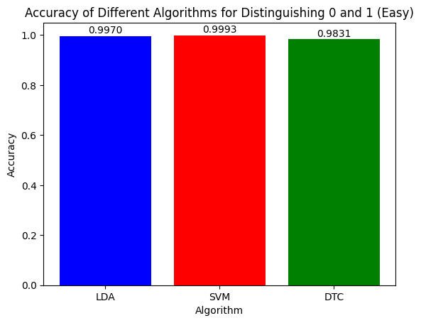 Figure 9: Accuracy of the Three Algorithms on Separating Easiest Pair (0,1)
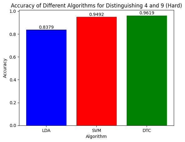 Figure 10: Accuracy of the Three Algorithms on Separating Hardest Pair (4,9)
Beginning with the easiest pair (0,1), all three algorithms did execptionally well with almost 100% accuracy for LDA and SVM and around 98% for DTC. This shows that all three algorithms can classify images that should be easy to easy to diffrentiate between very well.
However, when distingushing between the hardest pair (4,9), it is evident that DTC did the best with 96% accuracy. SVM did slightly worse with around 95% whereas LDA was comparatively significantly worse with only 84% accuracy. This shows how the intricacy of the SVM and DTC algorithms are more beneficial at separating between closely knit clusters in our PCA feature space. Additionally, we can definitely expect that if we had increased the number of PCA components, LDA would have attained a much higher accuracy as well.
Let us discuss and analyze the SVD feature space further:
 Figure 11: First 6 SVD Modes
The first 6 SVD modes are the first 6 columns of our U matrix that resulted from SVD. These modes tell us the direction in the input space along which the data varies the most up to the 6th most. These directions give us an idea of the most important patterns or features present in the MNIST data. In particular, the first few modes are often used for dimensionality reduction or feature extraction in machine learning tasks.
Thus, we can see that SVD Mode 0 defines the most important features in the dataset. It appears to look like a mix of a 9 and an 8 whereas SVD Mode 1 seems highly similar to a 0. Hence, we can see what SVD identified to be the features that would help classiify this data most accurately.
 Figure 12: First 6 V Modes
The first 6 V modes are the first 6 columns of our V matrix that resulted from SVD. These modes tell us the directions in the feature space (i.e., the space spanned by the columns of the data matrix) along which the data varies the most up to the 6th most.
Note that we did not truncate SVD and thus we ran it on 784 components. With such high (maximum) dimensionality, the V modes extract with pixels helped classify the data the most. It is difficult to interpret exactly why these pixels were chosen but it is still an intersting phenomenon to observe.
We then projected our data onto different sets of 3 V-modes and plotted in 3D:
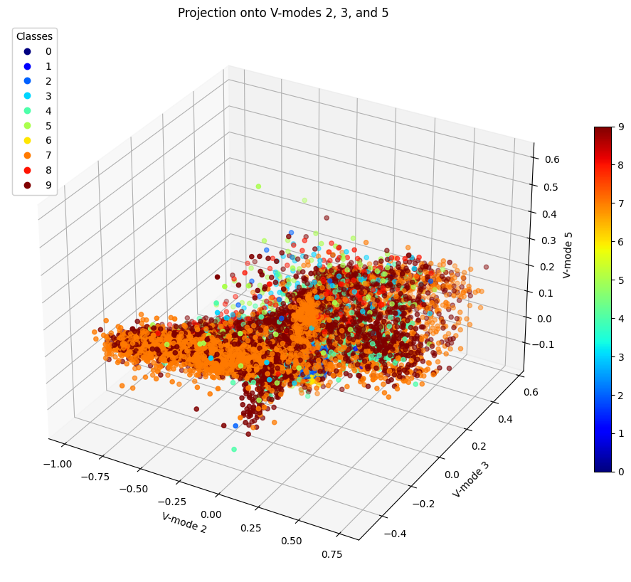 Figure 13: Projection of Data onto V-modes 2, 3, and 5
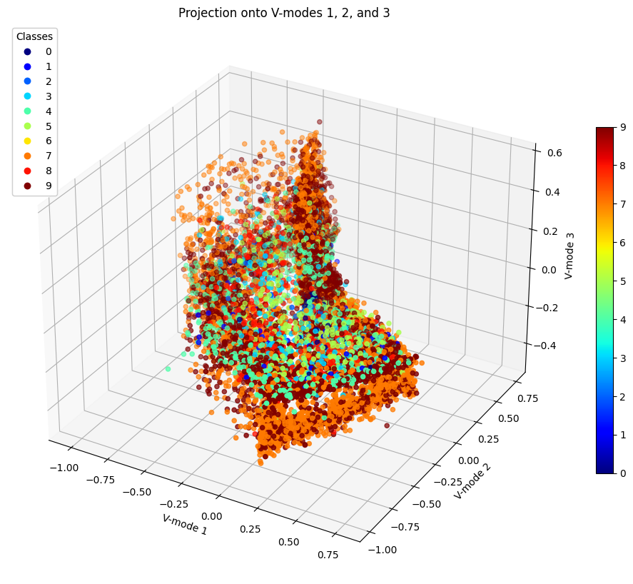 Figure 14: Projection of Data onto V-modes 1, 2, and 3
 Figure 15: Projection of Data onto V-modes 0, 1, and 2
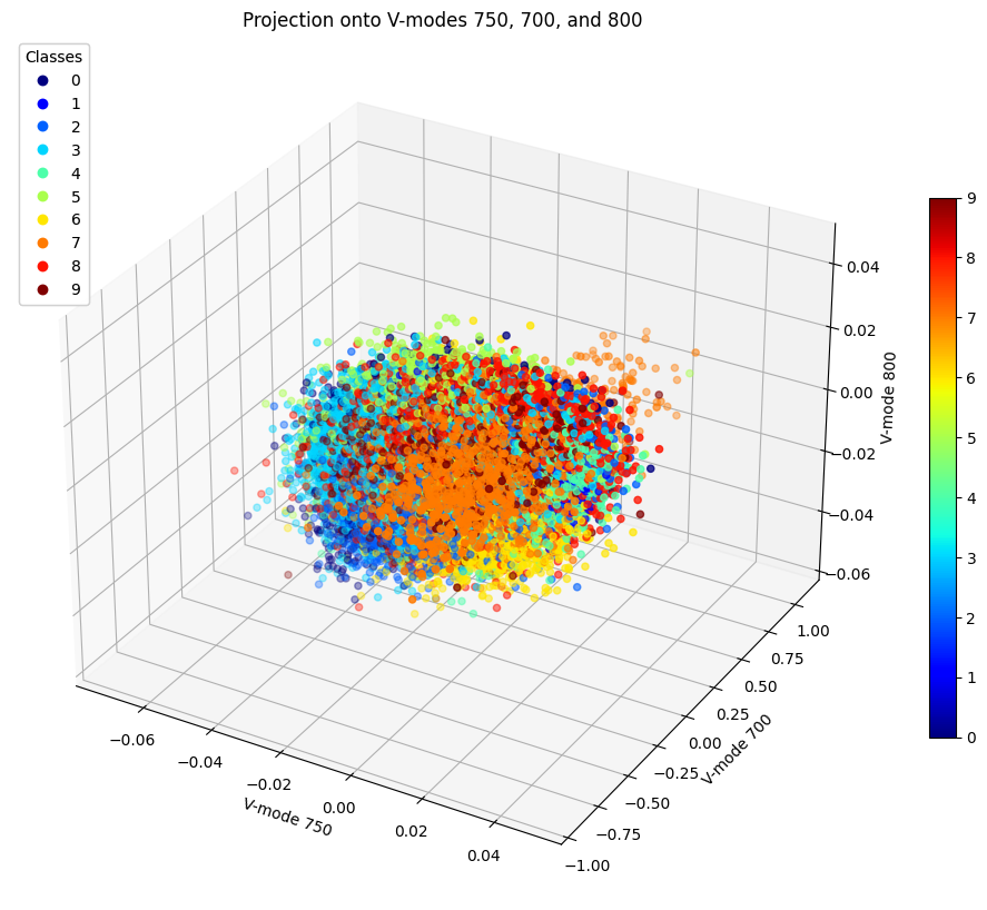 Figure 16: Projection of Data onto V-modes 750, 700, and 800
While we could not find three modes that would allow a clearer view of data clustering, we can still analyze these several cases altogether. We can see that typically 7 and 9 remain close to each other and in fact according to LDA, they were the 4th most difficult to separate with an accuracy of 91%. At least however they are more easily seperable than 4 and 9 which in all cases appear to be completley mixed into each other. This shows why it was so difficult to separate them using LDA since this problem was too difficult to solve using a linear analysis. Whereas using SVM for example, these points were moved to higher dimensions and cut by hyperplanes, thus provding a better classification accuracy.
In this project, we performed a detailed analysis of the MNIST dataset, which is a collection of handwritten digit images widely used in machine learning research. We started by performing an SVD analysis of the digit images and determined the number of modes required for good image reconstruction. We also interpreted the U, Σ, and V matrices in this context.
Next, we built a linear classifier (LDA) to identify individual digits in the training set. We determined which two digits in the data set were the most difficult and easiest to separate and quantified the accuracy of separation using LDA on the test data.
Finally, we compared the performance of LDA, SVM, and decision trees on the hardest and easiest pair of digits to separate. We found that LDA performed well on the easiest pair, but SVM and decision trees outperformed LDA on the hardest pair.
In conclusion, we successfully analyzed the MNIST dataset and demonstrated the effectiveness of SVD analysis and linear classifiers for identifying handwritten digits. We also compared the performance of different classification algorithms and found that SVM and decision trees can outperform LDA in some cases. Our analysis provides valuable insights into the strengths and weaknesses of different machine learning techniques for image classification tasks.