The technique of clustering in machine learning has found its way when the field was just starting to get hold in the world. Since then, there has been huge developments in the algorithms, techniques, and statistics that make up the art of clustering. The more it has found its way into the hearts of data science practitioners the more its resented due to its high sensitivity and ambiguous results which are subject to change based on initial parameters. The algorithms run so deep that there are heaps of research on how to tune its parameters to achieve a specific task. The initial position of centroids, random guess about the total number of initial clusters determined by extrinsic methods, tolerance, threshold, iterations, convergence, distance metrics, these are some of the parameters that can vastly effect the clustering results.
In the field of NLP and text analytics the datasets usually are textual documents from which hidden meaning are to be extracted. Numbered data is easily identified by the machine and computes the results quickly. Whereas textual data cannot be read by the machine because the semantic and syntactic meaning is lost on it. To overcome the problem, the document or a dataset is converted into more readable form like a matrix representation so that a machine could decipher it easily. The matrix representation of documents is a technique via which a document is molded into a matrix with respect to the terms present in it. Like clustering algorithms, there are several ways to achieve that. Most simple matrix that can be made from a document is a Binary-Frequency Matrix where each entry shows the presence of a particular term in a document. A matrix comprising of only zeroes and ones makes it one of the simplest mathematical representation of textual data. Furthermore, Term-Frequency Matrix is yet another example of mathematical representation of textual data where each entry of the matrix holds the number of times a specific term appears across all the documents. Both representations are quite simple and straight forward. There are other more sophisticated mathematical ways, that especially help in reducing the unwanted bias due to recurrent terms that appear in the other two methods. The formulation of TF-IDF or Term Frequency- Inverse Document Frequency Matrix is one of the most popular and widely recognized method of textual data representation.
One problem persists in parsing through mathematical representation of textual data and that is the problem of computation. In real world problems a machine is subjected to a huge number of data points to deal with. Making a matrix out of the data and performing operation on it requires very large number of resources and is highly inefficient. To counter the problem of complexity, it was found that a matrix can be divided into its constituents’ matrices which if combed together results in the same matrix. This type of method of matrix manipulation is known as Singular Value Decomposition. It divides the matrix into its constituents based on its eigen values and eigen vectors. Moreover, the matrix dimensions can further be reduced by keeping only those values or features that sufficiently describes the original data. The rank of the matrix is reduced such that it retains its most of the original information without much loss. The easiest way to achieve that is to use different values of rank and check whether significant loss of data occurs or not. Nonetheless, the method of SVD reduction has proved to be useful when dealing with textual data and documents.
The objective of this tutorial is to apply clustering and SVD on a data of news headlines to find out ideal pre-processing method, best number of clusters and optimum value of rank or k for SVD reduction.
Three different matrix representations (Binary, TF, TFIDF) of the data are used for the assignment to single out the best one among them. Each matrix representation creates a document-term matrix on which a series of functions are applied. The code first creates a document term matrix based on vectorization method used (either binary, TF or TFIDF). Then the matrix is subjected to different functions to create a scree plot, dendrogram and a silhouette curve to determine the number of clusters. Furthermore, the algorithm of affinity propagation is applied to the matrix to find yet another possible number of clusters. In addition, the matrix is subjected to the function that finds the ideal number of k or rank for SVD reduction. The ideal value for the rank reduction is then utilized further for topic modelling. In total, four different methods of cluster determination and two functions each finding the ideal rank value for reduction and then in turn applying topic modelling are used on each type of document term matrix pertaining to each different method of vectorization used. In the end all three vectorization methods are compared with each other to determine the best for clustering.
The python IDE used for the assignment is Anaconda’s distributed IDE named Spyder along with Python as the programming language. Furthermore, some of the important libraries and packages utilized for the task are newsapi, requests, spacy, numpy, sklearn, scipy, os and pandas.
As with any other data science task, procurement of the required dataset is the first and the most crucial step. The dataset used for this tutorial is of News Headlines related to any topic. The topic or keywords used to obtain the data are stored in a list named ‘keywords’ that holds few words according to which the news headlines are scraped and stored in a text file. Any number of topics can be added to the list ‘keywords’ and the function ‘News()’ will create a dataset containing all the news headlines related to all the topics listed in the ‘keywords’ variable. When the function ‘News()’ is called, it creates a text file of 500 news headlines which is then used for further analysis. If a file already exists, then it prints the message. Hence to create the file from scratch the file name ‘dataset.txt’ must be removed from the machine.
The pre-processing step for this assignment caters to the lemmatization, tokenization and removing of stop words of the dataset. Spacy’s pre-trained pipeline, en_core_web_lg is used to determine the stop words for the document. The function sw_tok_lemm takes the name of the text file of dataset as its parameter and performs the required tasks of pre-processing on the data. It stores the result in a variable called documents.
A binary or presence matrix is made via CountVectorizer() function to represent the dataset. This document term matrix has 500 rows where each row is a news headline from the dataset. The number of columns is more than 1000 on average representing the important terms from all the headlines.
TF matrix is made by using CountVectorizer() function with Boolean parameter binary set to False. It forms a document term matrix where each entry shows the actual number of times a term appears in the data.
TFIDF matrix is made by using TfidfVectorizer() function which outputs a document term matrix having combinational weights for each term.
The function scree_plot() makes an elbow curve for different number of clusters by plotting Squared Sum of Errors against the number of clusters. If the graph shows an elbow then the corresponding cluster is the output but if there is no definite elbow, then the cluster corresponding to the lowest number of SSE will be the output value for number of clusters as determined by the plot. The figures below show scree plots made for each document term matrix:
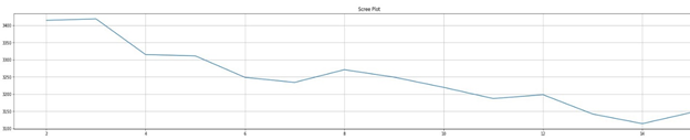
Fig.1 - Scree Plot of Binary Document Term Matrix
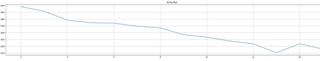
Fig.2 - Scree Plot of Term Frequency Document Term (TF DT) Matrix
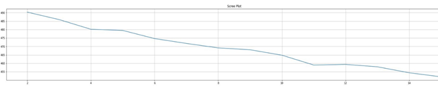
Fig.3 - Scree Plot of Term Frequency - Inverse Document Frequency Document Term (TFIDF DT) Matrix
As shown from the above figures neither of the plots have a prominent single elbow. It may result due to the nature of the dataset. If the initial keywords used to make the dataset are changed, maybe a better plot can be made.
The function dendogram_() makes a dendrogram for binary and TF matrices only. For TFIDF matrix, another function, dendogram_tfidf() is used. It is because of the relative distance from the root to the leaves in both dendrograms are different. Hence to draw a correct line, at correct height across the dendrogram requires different lines of codes for TFIDF and the other two matrices. The ideal numbers of clusters from the dendrogram are the output for both functions along with the drawn graphs. The figures below show the dendrogram for each document term matrix:
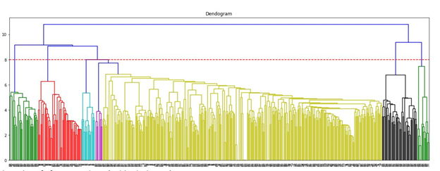
Fig.4 - Dendogram (Binary DT Matrix)
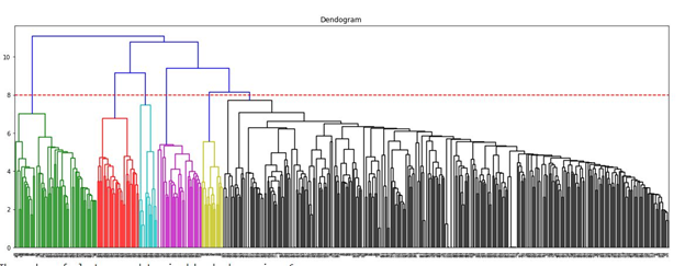
Fig.5 - Dendogram (Binary TF-DT Matrix)
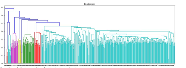
Fig.6 - Dendogram (TFIDF DT Matrix)
The function silhouette_() plots average silhouette coefficient against number of clusters for the three documents term matrices. The maximum silhouette from the graph resulting from its corresponding number of clusters is taken as the output of the function. The figures below show the silhouette curve for all three document term matrices:
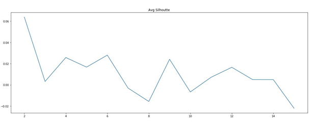
Fig.4 - Silhouette Curve (Binary DT Matrix)
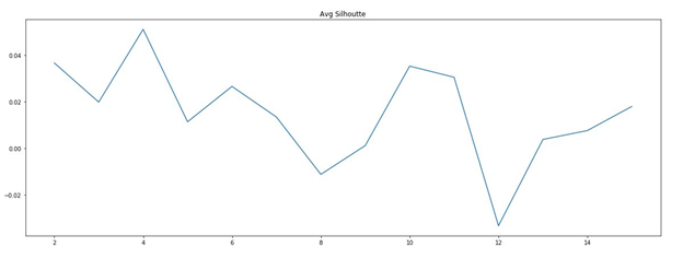
Fig.5 - Silhouette Curve (Binary TF-DT Matrix)
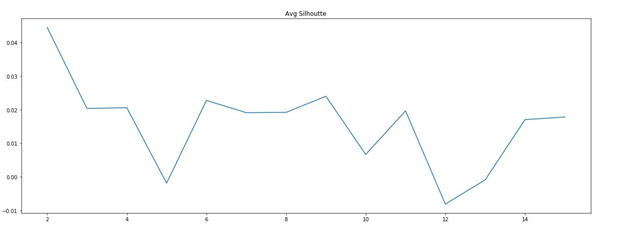
Fig.6 - Silhouette Curve (TFIDF DT Matrix)
The algorithm of affinity propagation is applied to each of the matrices to find the ideal number of clusters. The function affinity_prop() runs the AP algorithm and predicts the number of clusters suitable for the problem. It may happen that the output results in convergence error. It means that the algorithm has failed to converge the matrix and hence cannot predict the number of clusters. If that happens, the parameters of AffinityPropagation function of sklearn library must be tuned so that a convergence may occur. The parameter random_state can be set to any integer for reproducibility of results. The output of the user defined function affinity_prop() is the number of clusters as predicted by the AP algorithm.
The algorithm of clustering is applied on each of the document term matrix. For each matrix the cluster_() function applies clustering with number of clusters equal to each value determined by scree plot, dendrogram, silhouette and affinity propagation. The cluster_() function takes a matrix for its parameter along with four n_cluster values found via methods described above. The four n_cluster values are then used one by one in clustering algorithm. The silhouette score for each time a clustering algorithm is run for n_cluster is stored in a list. The output of the cluster_() function is the best number of clusters for the document term matrix in consideration on the basis of maximum silhouette score.
The ideal value for reduced rank for truncated SVD is found for each document term matrix via ideal_k() function. The easiest way to go about finding the ideal value is to run a hit & trial method. This process may sound easy but is quite inefficient. The reason for reducing the original document term matrix is to make it computationally easy yet retaining useful original information. Sometimes unnecessary reduction results in loss of data which in turn provides poorer results. To cater to the problem of information loss and matrix reduction a new metric named ratio of variance explained is used. It is an attribute of an object formed via TruncatedSVD function. This metric tells us the amount of variance explained of the original data by the reduced matrix. 70% is taken as threshold value. If at any value of k or rank, the reduced matrix can explain 70% of the variance of the original data, then that value of k is marked as ideal. As we increase the value of k, the number of features (term) are also increased. Which in turns increases the amount of variance explained, until a value of k is reached such that the variance explained is almost 70%. For example, n_components equal 100 (in our case the total features are more than 1000 so an initial value of 100 is understandable) gives out 50% as total variance explained, then we will add another few features and check the variance again which will be greater than that of 100 features. Each addition of the feature makes the reduced matrix approximation closer to the original. Building on this explanation, the function ideal_k() checks at what value of k the variance of the data is explained at least 70% and outputs it as ideal value of k, rank or n_components.
The final output of the function results() is the best overall matrix representation method among binary, TF and TFIDF on the basis of their performance judged by how well they have performed in clustering task. In addition to that it also prints the optimum number of clusters used for the best overall performance. In this case the best overall performance comes out for TFIDF matrix, but it can change depending upon the type of dataset created in the first place.
This project provides a code to read a document, pre-process it, create its matrix representation based on different methods of vectorization, finds the ideal number of clusters and rank for SVD and tries as a proof of concept to model the topics. The results may differ due to random_state parameter being uninitialized, but the code outputs the correct results whatever the data is, as it is written generically.