Home
Note: the user manual pdf contains the same information as below, but is more up-to-date and has better formatting.
The Universal Probe Finder is a multi-species histology processing and probe alignment pipeline. It can read multiple ephys formats so you can use neurophysiological markers to better fine-tune your probe’s location in the brain. It can use multiple atlases and calculates the stimulus responsiveness of your clusters with the zetatest using only an array of event-onset times.
The pipeline consists of three modules:
- SlicePrepper: annotate where the probes left tracks on your histology slices,
- SliceFinder: align your histology slices to the brain atlas,
- ProbeFinder: fine-tune your probe’s location based on neural response markers.
At this time, the Universal Probe Finder supports the following atlases out-of-the-box: a. Sprague Dawley rat brain atlas, downloadable at: https://www.nitrc.org/projects/whs-sd-atlas b. Allen CCF mouse brain atlas, downloadable at: http://data.cortexlab.net/allenCCF/ c. CHARM/SARM NMT_v2.0_sym macaque brain atlas: https://afni.nimh.nih.gov/pub/dist/doc/htmldoc/nonhuman/macaque_tempatl/atlas_charm.html
Moreover, it currently supports the following ephys formats: a. Clustered spiking data from Kilosort, downloadable at: https://github.com/MouseLand/Kilosort b. Raw SpikeGLX data, downloadable at: https://billkarsh.github.io/SpikeGLX/ c. Acquipix pre-processed data, downloadable at: https://github.com/JorritMontijn/Acquipix
It is also possible to add your own ephys format or atlas: see the section “Adding an atlas”/”Adding an ephys format”.
- For best performance, make sure your GPU supports OpenGL-accelerated graphics, so update your drivers if required.
- Download the brain atlas you wish to use, for example: a. Sprague Dawley rat brain atlas: https://www.nitrc.org/projects/whs-sd-atlas b. Allen CCF mouse brain atlas: http://data.cortexlab.net/allenCCF/ c. CHARM/SARM macaque brain atlas: https://afni.nimh.nih.gov/pub/dist/doc/htmldoc/nonhuman/macaque_tempatl/atlas_charm.html#download
- Install the atlas if required (i.e., extract the files to nifti/.nii)
- All required external files are included in the repository’s subfolders so you only need to clone this repository: https://github.com/JorritMontijn/UniversalProbeFinder
- Add the main path to matlab and you’re done – or, as the English would say: Bob’s your uncle! Note: if you do not clone the repository, but instead download the files as a .zip package from github.com, you will have to also download the zetatest submodule manually, as this submodule will not be automatically included in the zip file.
Once you have downloaded the atlas you wish to use (see above) and the Universal Probe Finder repository, it’s very easy to start. Open matlab and navigate to where you installed the repository (replace the path with wherever it is on your PC): cd F:\Code\Acquisition\UniversalProbeFinder Next, simply type UniversalProbeFinder, and it will start the program: UniversalProbeFinder It will then ask you which program you would like to run: The SlicePrepper, the SliceFinder, or the ProbeFinder. If you want to annotate your histological slices with electrode tracks, start with the SlicePrepper. If you already have a probe coordinate file, or simply wish to plan your implantation trajectory, start with the ProbeFinder.
When starting the SlicePrepper, you can select the folder from where you want to import your slice images or load your previous data. For example, in a folder where there are already prepared and aligned the slices, you can see something like:
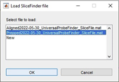
You can load either the prepped or the aligned data, or start from scratch and import the images from your selected folder. If you click “New”, you can then select and reorder which images you would like to import. Once you’re happy, click “Accept”. The SlicePrepper will now process your images. The first thing you want to do for each slice is to align the midline to vertical. Push the Control button and left click somewhere along the top of the midline, then select a second point below it to adjust your slice orientation. Next, you can create a new track by clicking on “New” in the track selector panel. You can now give your track a name, a marker and a colour. Once you have created a track, you can draw a trajectory on the slice by left clicking once to a beginning point, and again left clicking to set the end point:
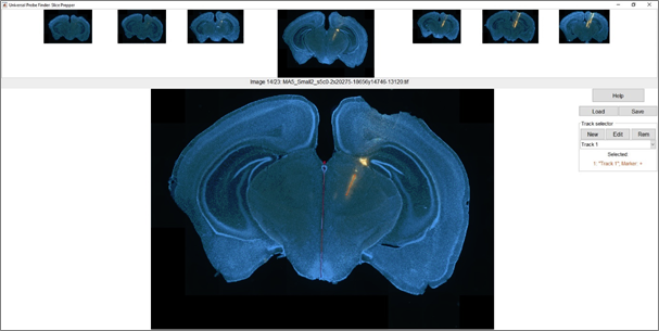
To navigate through your slices, you can use the left/right arrows, page up/down, and home/end. You can also swap the position of the current slice with the previous or next slice by using shift + left/right arrow. Once you have set all the tracks in your slices, you can click “Save” to save the data and continue in the SliceFinder.
Load your data folder as with the SlicePrepper and select the Prepped(…) file to load the tracks you annotated on the images. You will now also be asked to select which atlas you wish to use, which by default is either mouse, rat, or macaque:
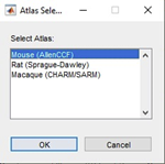
If this is the first time you’re starting the SlicePrepper or ProbeFinder, it will now ask you where you installed the atlas you selected. Navigate to its directory and click OK. In the SliceFinder you can move, rotate, and rescale the slices with respect to the atlas. When you start the SliceFinder, all slices will be set to the middle of the atlas on the DV and ML axes, and to the AP position that matches the origin of the atlas (e.g., bregma):
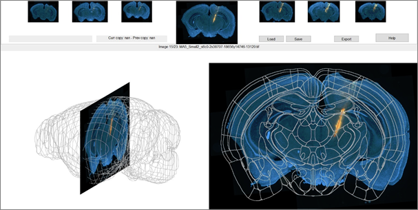
While you can align each slice one by one, a more efficient approach is to align one slice at the beginning of the range you’re interested in, and align one slice at the end, then interpolate the positions + rotations of the intermediate slices. You can copy a slice with control+c (e.g., slice #10), navigate to a different slice, copy this second slice by pressing control+c again (e.g., slice #20), and then press control+b to interpolate slices 11-19 based on the positions of slices #10 and #20. Assuming your slices are of similar thickness and they’re correctly ordered, this should set all slices close to their true position in a couple of button presses. If you ever make a mistake, you can undo your last paste action (control+v or control+b) by pressing control+z.
When starting the ProbeFinder, select your atlas. If you wish, you can now also import:
- A probe file of various formats, such as: a. AP_histology output b. SHARP-track output c. ProbeFinder output
- Electrophysiological data, such as: a. A kilosort 2.5 or kilosort 3 output folder b. SpikeGLX raw data c. Spike-detected ProbeFinder data
- An event-time or cluster-responsiveness file, such as: a. A matlab file containing event onset times b. An Acquipix file c. A file containing ZETA responsiveness values If you load raw SpikeGLX data, the ProbeFinder will first run spike detections on all channels to convert the data to multi-unit spike times. You can save this pre-processed data for later use so you don’t have to run the spike detections again. Similarly, if you select unprocessed event times for your responsiveness file, it will compute the neural responsiveness per cluster or channel based on the spike times and the event onsets you provided with the zeta-test (https://elifesciences.org/articles/71969). When it’s done, you can save the file for future use.
Once you’ve loaded a probe, ephys, and responsiveness file, you will see something like:
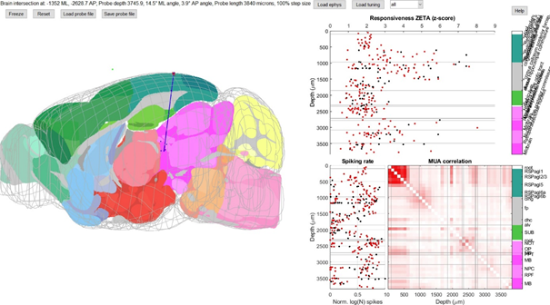
On the left, you can see an outline of the brain and a slice somewhat orthogonal to your viewing direction that goes through the probe. If you imported a probe location file, you will see blue dots that indicate where you thought the probe tracks were located on your histology slices. The green dot floating outside the brain is Bregma. Normally, this histology-based location is what you would export and use to assign areas to the clusters you recorded on your probe. But often this is not entirely correct! As you can see above, the depth is clearly wrong, but only moving the probe up is not giving a good match either. The spiking rate and the MUA correlation (bottom right) give a pretty good indication of where the top of the cortex is located (MUA correlation is strong for noisy contact points above the brain) and where the white matter bundles lie (clusters show low firing rate). The exact boundaries between different cortical and subcortical areas are more difficult to determine, however. In this experiment, I showed drifting gratings and natural movies, so calculating the responsiveness ZETA scores using their onset times shows a clear delineation of visually-responsive and non-visually responsive regions (top right). Tweaking the probe location, length and angle a bit, I ended up with this alignment (not perfect yet, but clearly a lot better than before):
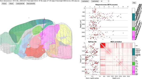
Notice how the subiculum has a high MUA correlation, the NOT has a couple of highly visually-responsive cells, and the boundaries of the visual cortex are very sharp when looking at the responsiveness ZETA. When you’re happy with your alignment, you can click on “save probe file” and export the current location. The ProbeFinder will then calculate for each cluster what its area in the brain is, according to your atlas.
The initial probe location is calculated from a set of points in atlas-space. In order for the ProbeFinder to read a file successfully, the file should contain the variable “sProbeCoords” with at least:
-
cellPoints [1 x N]: cell array where each cell contains points for a single probe i, i.e.:
o cellPoints{i} [P x 3]: P points with [ML AP DV] native-atlas format coordinates You can also add the following optional field to supply a name for each probe:
-
cellNames [1 x N]: cell array where each cell contains the probe’s name
Note that if you use the SlicePrepper and SliceFinder, these files are automatically generated when you click the “Export” button.
The current probe location is saved in the field “sProbeAdjusted” of the structure “sProbeCoords”. The sProbeAdjusted structure contains the following fields, of which the more useful fields are marked in bold: -probe_vector_cart [2 x 3]: cartesian tip and base coordinates in [ML,AP,DV] atlas space -probe_vector_sph [1 x 6]: spherical coordinates: [ML AP DV deg-ML deg-AP length] -probe_vector_intersect [1 x 3]: coordinates of brain entry -probe_vector_bregma [1 x 6]: bregma-origin format: [ML AP ML-deg AP-deg depth length] -probe_area_ids_per_depth [1 x N]: vector of area IDs per point along the probe -probe_area_labels_per_depth [N x 1]: cell array of acronyms per point -probe_area_full_per_depth [N x 1]: cell array of full names per point -probe_area_boundaries [1 x P+1]: locations along the probe of area boundaries -probe_area_centers [1 x P]: centers of areas -probe_area_ids [1 x P]: id per area of the above -probe_area_labels [P x 1]: acronym per area -probe_area_full [P x 1]: full name per area -stereo_coordinates: table with the probe’s location in stereotactic coordinates: Name: Content: Unit ML Probe’s brain entry location along ML (medial-lateral) axis, relative to the atlas origin (e.g., bregma) Microns AP Probe’s brain entry location along AP (anterior-posterior) axis, relative to the atlas origin (e.g., bregma) Microns Angle_ML Angle of the probe in the ML direction (see below) Degrees Angle_AP Angle of the probe in the AP direction (see below) Degrees Depth Depth below the brain entry of the lowest recording channel of the probe (i.e., usually the depth of the tip) Microns Probe_Length Length of the probe after stretching/shrinking Microns
-probe_area_ids_per_cluster: area IDs per cluster -probe_area_labels_per_cluster: area acronyms per cluster -probe_area_full_per_cluster: full name of the area per cluster Note that these final three _per_cluster variables only have values if electrophysiological data was loaded when the probe file was saved.
Defining a single axis of 360-degree rotation in R3 is trivial and defines a unique set of points. Unfortunately, combining two 360-degree axes of rotation in 3-dimensional space leads to a non-unique spherical projection space, where multiple combinations of the two angles describe the same point. Describing these problems in detail is beyond the scope of this manual (see https://en.wikipedia.org/wiki/Spherical_coordinate_system#Unique_coordinates for more details), but it is important to note that converting between cartesian and spherical coordinate systems can be tricky. For our purposes of defining a probe’s location, it is most useful to have two axes that align more or less with our two most important axes: ML and AP. Moreover, a natural “origin” for the probe would be to define the direction going straight down as 0 degree ML and 0 degree AP. This requires rotating the spherical coordinate system (fig. 1).
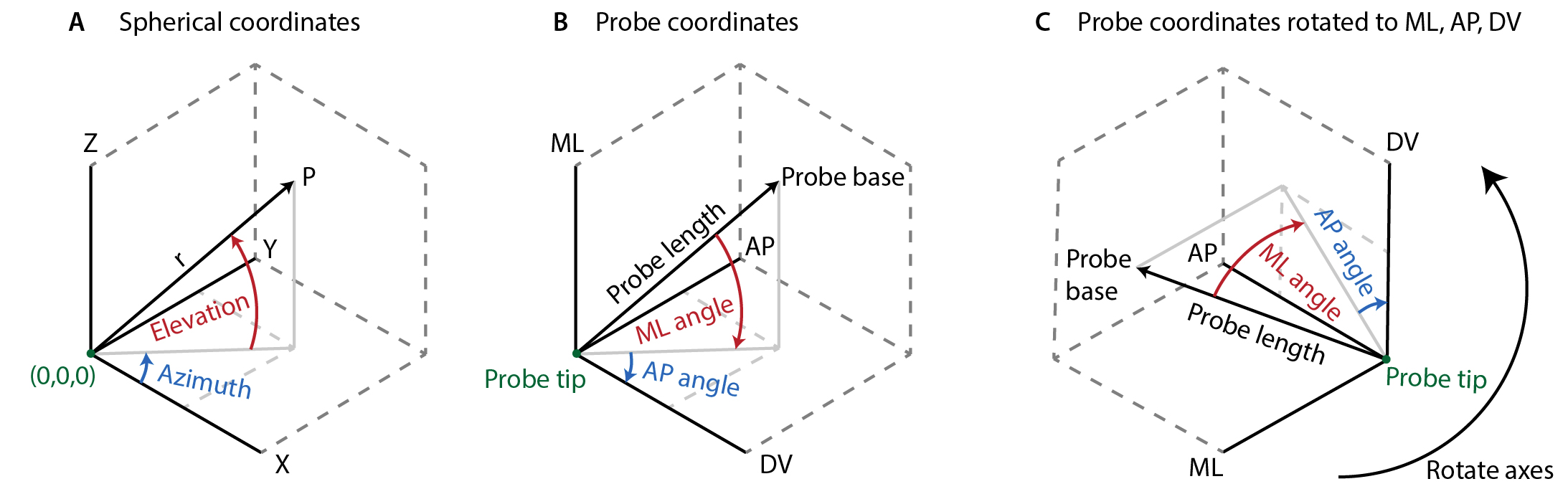
Figure 1. Definition of ML and AP angles. A) Standard spherical coordinate system using elevation and azimuth. Azimuth is defined on the interval [-π, π] and elevation on [-π/2, π/2]. B) X,Y,Z, replaces by stereotactic axes. Notice the change in angle direction. C) Rotated axes aligned with atlas directions. Furthermore, to ensure that the necessary discontinuities in the rotations occur when the probe is upside-down (which presumably is not a common recording orientation), rather than close to its “origin” position, we invert the AP-axis and apply the following transformations:
if dblAngleAP < -90 && dblAngleML > 0
    dblAngleAP = dblAngleAP + 180;
    dblAngleML = -dblAngleML + 180;
elseif dblAngleAP < -90 && dblAngleML < 0
    dblAngleAP = dblAngleAP + 180;
    dblAngleML = -dblAngleML - 180;
elseif dblAngleAP > 90 && dblAngleML > 0
    dblAngleAP = dblAngleAP - 180;
    dblAngleML = -dblAngleML + 180;
elseif dblAngleAP > 90 && dblAngleML < 0
    dblAngleAP = dblAngleAP - 180;
    dblAngleML = -dblAngleML - 180;
end
The specific implementations can be found in the functions PH_CartVec2SphVec, PH_SphVec2CartVec, PH_BregmaVec2SphVec, and PH_SphVec2BregmaVec.
The ProbeFinder reads a configuration .ini file to find which atlases are installed. If no configAtlas.ini file is present, it will create a default file containing metadata on the Allen Brain mouse atlas, Sprague-Dawley rat atlas, and CHARM/SARM macaque atlas. If you wish to add an atlas, you can edit the .ini file by adding another atlas entry set. For example, the first entry looks like this: [sAtlasParams(1)] name='Mouse (AllenCCF)' pathvar='strAllenCCFPath' loader='AL_PrepABA' downsample=2
It specifies:
- name: the name of the atlas,
- pathvar: the name of path variable that is saved in configPF.ini (the atlas’s path location)
- loader: the name of the function that pre-processes the atlas files (see below)
- downsample: the amount of downsampling when plotting an atlas slice The name, pathvar, and downsample are self-explanatory, but the loader requires some more explanation. The syntax of a loader function is: sAtlas = name_of_loader_function(str_atlasname_Path)
The loader function reads the atlas files at the specified path and outputs a structure sAtlas with the following fields: Field name Size Description .av [ML x AP x DV] Annotated volume, where a value in av denotes an area ID that can directly index into .st; i.e., sAtlas.st(sAtlas.av(x,y,z)).name gives the full name of the area at location x,y,z. .tv [ML x AP x DV] Grey-scale template volume in range [0 255] .st [N x T] table N-entry table, where N is highest area index in .av .Bregma [1 x 3] Origin of atlas in native atlas voxel coordinates [ML AP DV] .VoxelSize [1 x 3] Size of a single voxel in microns [ML AP DV] Note: currently only isometric voxels are supported .BrainMesh [P x 3] Mesh of brain outline, where each vertex is a [1 x 3] point, and curve-ends are denotes by a [nan nan nan] entry. Brain meshes can be created from a .av or .tv volume using getTrace3D .Colormap [N x 3] N-entry RGB color map, specifying a color for each area in .av .Type string Name, e.g.: Allen-CCF-Mouse
The area-table .st must have least the following fields: Field name Description st.id ID of area (numeric) st.name Full name of area (string) st.acronym Short name of area (string) st.parent_structure_id ID of parent area
If you wish to add an atlas to the program, we are happy to help out. You can contact us by e-mail or via the github repository.
Adding an electrophysiology format Similar to when loading an atlas, the ProbeFinder reads a configuration .ini file to find which ephys formats are installed. If no configEphys.ini file is present, it will create a default file containing metadata on Kilosort, SpikeGLX, Acquipix, and the native ProbeFinder ephys format. If you wish to add a format, you can edit the .ini file by adding another entry set. For example, SpikeGLX’s entry looks like this: [sEphysParams(2)] name='SpikeGLX' loader='EL_PrepEphys_SG' reqfiles='.[.]imec.[.]ap[.]bi+n,.[.]imec.[.]ap[.]met+a,.[.]nidq[.]bi+n,.[.]nidq[.]met+a' reqisregexp=1
It specifies:
- name: the name of the format,
- loader: the name of the function that pre-processes the format (see below)
- reqfiles: comma-separated list of files that must be present for the format to be valid
- reqisregexp: specified whether the file names are regular expressions or plain-text Most formats will need to use regular expressions, as the filenames can change between recordings. However, in the case of kilosort for example, it always produces the same set of file names, so these must be an exact match; and therefore the switch reqisregexp will be 0. The loader function reads the ephys files at the specified path and outputs a structure sClusters: Field name Size Description .dblProbeLength [1 x 1] Length of the probe in microns .vecUseClusters [1 x N] Cluster id, where N is the number of used clusters/channels .vecNormSpikeCounts [1 x N] Spike counts per cluster, by default: mat2gray(log10(S+1)) .vecDepth [1 x N] Depth below base of probe per cluster/channel .vecZeta [1 x N] Zeta-responsiveness values (or contamination) .strZetaTit [string] If no zeta values are present, this is 'Contamination (%)' .cellSpikes [1 x N] Spike times per cluster/channel .ClustQual [1 x N] Quality index per cluster .ClustQualLabel [1 x N] Label per cluster (“mua”, “good”) .ContamP [1 x N] Contamination percentage per cluster If you wish to add a format to the program, we are happy to help out. You can contact us by e-mail or via the github repository.
Acknowledgements This work is based on earlier work by people from the cortex lab, most notably Philip Shamash and Andy Peters. See for example: https://www.biorxiv.org/content/10.1101/447995v1 This repository includes various functions that come from other repositories, credit for these functions go to their creators: https://github.com/petersaj/AP_histology https://github.com/JorritMontijn/Acquipix https://github.com/JorritMontijn/GeneralAnalysis https://github.com/kwikteam/npy-matlab https://github.com/cortex-lab/spikes https://github.com/JorritMontijn/zetatest If you use the Universal Probe Finder, please cite our paper.
Good luck probe finding! Troubleshooting Question (“actually, it’s more of a comment”): It doesn’t work Answer: Restart your PC, make sure the UniversalProbeFinder is on your matlab path, and try again.
Q: The program crashes because it says it’s missing a file? A: You’ve probably downloaded the code a zip file (see “Installation Instructions”). If you do this, the zetatest module and its dependencies are missing. If you download and extract the zetatest repository manually, it should probably fix your problem. If not, please make a bug report on github.
Q: Why is it so slow? A: You’re probably not using OpenGL rendering. If you’re from the future, your matlab version might have broken the OpenGL rendering switch. If so, please file a bug report. If you’re using anything that’s R2022a or earlier, you might need to update your GPU or your graphics drivers.
Q: I’m using R2022a or earlier, updated my drivers, have a compatible GPU, and it’s still slow. A: It’s possible that the atlas slices are slowing things down. If hiding the slices with “s” speeds things up, you might want to consider editing the configAtlas.ini file to increase the downsampling for your atlas (Note: values are rounded to the nearest integer). For example, if you’re using the Allen Brain atlas, you will see: [sAtlasParams(1)] name='Mouse (AllenCCF)' pathvar='strAllenCCFPath' loader='AL_PrepABA' downsample=2
You can change the line “downsample=2” to (e.g.) “downsample=5”, restart the ProbeFinder, and see if it makes a difference.
Q: I found a bug A: If you’ve fixed it, you can make a pull request, otherwise you can create a bug report here: https://github.com/JorritMontijn/UniversalProbeFinder/issues. Please copy/paste the error message and provide as much detail as you can about what you were doing when it happened. If I cannot recreate the issue, I probably won’t be able to fix it.