What is EEG-Pype?

With our software, we hope to provide users with an accessible way to preprocess resting-state EEG files, while still including powerful analysis tools. We do this by combining several functions from the MNE (MEG/EEG preprocessing) open-source project (Gramfort et al., Frontiers in Neuroscience, 2013). Inspiration was taken from BrainWave as well (https://github.com/CornelisStam/BrainWave), especially for the quantitative analysis module. By using an intuitive graphical user interface on top of a Python script, we hope that our software is easy to start using without coding experience, while still allowing more experienced users to adapt the software to their needs by altering the underlying code.

The software is currently able to:

• Open raw EEG files of types supported by MNE's mne.io.read_raw() function.
• Open a single EEG or choose analysis settings for an entire batch of files.
• Apply a montage to the raw EEG (including electrode coordinates necessary for some analyses).
• Drop bad channels entirely.
• Interpolate bad channels after visual inspection.
• Apply an average reference.
• Apply independent component analysis to remove artefacts. For this, you can change the number of components that are calculated (please read up on this before use).
• Apply beamformer source reconstruction to the EEG (standard MNE LCMV beamformer with standard head model).
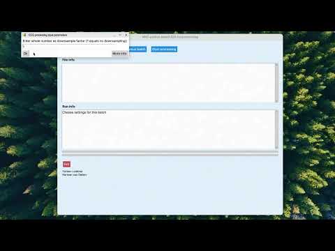
• Down sample the file to a lower sample frequency by specifying a downsample factor (like a factor of 4: from 2048 Hz to 512 Hz for example).
• Perform interactive visual epoch selection.
• Perform filtering in different frequency bands and broadband output. These bands can be changed for the current batch in the GUI or more permanently in the settings file (see under tips and issues). The EEGs are filtered before cutting epochs, reducing edge artifacts.
• Split alpha and beta bands into sub-bands (alpha1/alpha2 and beta1/beta2) for more detailed frequency analysis.
• After performing analyses on a batch, rerun the batch with preservation of channel and epoch selection. To do this, select the previously created .pkl file.
• Log the chosen settings and performed analyses steps in a log file.
• Correct channel names to match expected montage names through an interactive find/replace interface.

The software is not (yet) able to:

• Analyse task EEG data.
• Analyze MEG data.

In addition, a separate quantitative analysis module allows for the calculation of several commonly used quantitative measures on the resting-state EEG epochs that are created by our pre-processing module. See below for more details.

Tips for use and known issues

When choosing the settings for the current analysis batch, most windows contain a "more info" button which will take you to an appropriate MNE documentation page.

When no raw EEG files show up in the file selection window, please choose a different file type in the dropdown menu on the right (it might be stuck on only showing .txt files for instance).

For the bad channel selection (for interpolation), you can select bad channels by clicking the channel names on the left side of the plot. The deselected (grey) channels will be interpolated. For ICA, this works the same but then artefact-containing components can be deselected in the graph plot of the ICA. These components will be filtered out of the EEG. For interactive epoch selection, epochs of insufficient quality can be deselected by clicking anywhere on the epoch, which will then turn red. This means the epoch will not be saved.

We have added support for MNE's ICALabel functionality, helping the user along by providing predictions of what type of activity the independent components correspond to (i.e., different types of artifacts or brain activity). This prediction is based on a machine learning model, and the prediction is accompanied by a prediciton certainty percentage. See also their website.

If the program glitches or stops working, we found that it works best to stop the Python process, for instance by clicking the red stop button or restarting the kernel in Spyder IDE or similar.

When using Spyder IDE to run the program, initially Spyder can prompt the user that it does not have the spyder-kernels module. Please follow the instructions provided in the console.

It is possible to change the underlying Python code (however, this is mostly unnecessary). Of the two main scripts, eeg_processing_script.py and eeg_processing_settings.py, the latter is the easiest to modify. Here, you can for instance rather easily change the standard output filter frequency bands (like delta, theta etc.). Note however, that it is currently not possible to increase or decrease the number of bands that the output is filtered in. In some IDE's, or with certain setups, it can also be necessary to change the matplotlib backend, for instance from TkAgg to Qt5Agg in the beginning of the settings script.

If running the main preprocessing module (i.e, eeg_processing_script.py) from an IDE like Spyder does not work, there is also the option to run the script directly from the command line, in the same way as EEG-Pype's quantitative analysis module is run (see below in the Quantitative analysis module section for an explanation on how to do this).

When loading EEG files, the software includes a channel name correction feature. This helps when your EEG files have channel names that don't exactly match the expected montage (e.g., channels prefixed with "EEG" or having different capitalization), even though recognition of channel names is necessary for correct montage application. The interface shows you the current channel names versus the expected names for your chosen montage, and allows you to use find/replace to correct them. These corrections are then applied to each file separately. This way, there is a check for each file to see whether the channel names match the MNE montage.

When plotting the EEG channels side by side, note that ECG channels should be purple if recognized correctly: If this is not the case, these channels might be included in operations like average referencing.

The frequency band settings now include the option to split the alpha band (into alpha1: 8-10 Hz and alpha2: 10-13 Hz) and beta band (into beta1: 13-20 Hz and beta2: 20-30 Hz). You can toggle these splits when setting up your batch processing (under the change filter bands option). This allows for more detailed analysis of specific frequency ranges.

Additionally, there is also an option to include a custom frequency band in the GUI during setup of preprocessing. Leaving these fields empty will mean this band is ignored instead.

Short video overviews

Installation

This guide is designed for users who may not be familiar with coding or command-line tools. We will set up a virtual environment to keep all the software for EEG-Pype organized and install the necessary software step-by-step. Note: You only need to do steps 1 through 4 once.

1. Install the necessary tools

• Install Miniconda: Miniconda is a tool that manages the Python coding language for us. Miniconda Download link.

  • Windows: Under "Windows" download the "Windows 64-Bit Graphical Installer". Open the file and click "Next" through the installation. Important: If asked, leave the default settings as they are.
  • macOS: If you have a newer Mac (M1-M5 chips): Under "Mac" and "Miniconda" download the 64-Bit (Apple silicon) Graphical Installer. If you have an older Mac (Intel chip): Under "Mac" and "Miniconda" download the 64-Bit (Intel chip) Graphical Installer.
  • Linux: Install Miniconda by downloading the Linux installer from the same page.

• Install Git: Git allows you to download the software from this website.

  • Windows: Download and install Git for Windows ("Standalone Installer" then "x64" for most users unless you have an ARM-based CPU). During installation, you can keep clicking "Next" to accept all default settings.
  • macOS: Git is usually installed automatically on Mac computers. To check, you can skip this step for now; if you need it later, your Mac will prompt you to install it.
  • Linux: Git is usually pre-installed. If not, run sudo apt install git (Ubuntu/Debian) or sudo dnf install git (Fedora).

2. Download the EEG-Pype Code

• Open your command tool:

  • Windows: Open Anaconda Prompt (Miniconda3) (Do not use the standard Command Prompt/cmd).
  • macOS: Open Terminal.

• Copy and paste the following command into that window and press Enter:

git clone https://github.com/yorbenlodema/EEG-Pype.git

This downloads the EEG-Pype folder to your user folder.

3. Create the Environment

Now we will create the virtual environment or "sandbox" where the software is installed. This environment contains all packages (dependencies) that EEG-Pype relies on.

• To enter the correct folder, copy and paste this command and press Enter:

cd EEG-Pype

• To create the virtual environment, copy and paste this command and press Enter:

conda env create -f Environment.yml

Note: This step requires internet and may take a little while. You will see lines of text scrolling; this is normal.

• To activate the environment we just made, run this command:

conda activate EEG-Pype

Check: Look at the left side of your command line. It should now say (EEG-Pype) instead of (base).

4. Running the Software

Now that everything is installed, here is how you open the software. Make sure in Anaconda Prompt (Windows) or Terminal (Mac) you see (EEG-Pype) as the first thing on the last line, instead of (base). Seeing (EEG-Pype) here means that we have moved to or activated our virtual environment, containing the packages/dependencies EEG-Pype needs.

• Open Anaconda Prompt (Miniconda3) (Windows) or Terminal (macOS).
• Activate your environment by typing:

conda activate EEG-Pype

• Navigate to the source folder:

cd EEG-Pype/src

Or if you were already in the EEG-Pype folder:

cd src

• Run the preprocessing program:

python eeg_processing_script.py

Or run the quantitative analysis module:

python eeg_quantitative_analysis.py

You can also choose to open and edit the scripts included in EEG-Pype in a code editor like Spyder or Visual Studio Code. While running the scripts from the command line gives the most stable performance, the eeg_processing_script.py script can also be run from your code editor. For the eeg_quantitative_analysis.py script, we have found that currently, only running from the command line is possible.

Summary for Daily Use

Next time you want to use the software, you only need to do this:

1. Open Anaconda Prompt (Windows) or Terminal (Mac).
2. Type: conda activate EEG-Pype
3. Type: cd EEG-Pype/src
4. Type: python eeg_processing_script.py

For any issues, please feel free to open an issue on the GitHub repository.

Updating the Software

When there's an update available on GitHub, follow these steps to update your local installation:

1. Navigate to the Project Directory Open a terminal (or Anaconda Prompt on Windows) and navigate to your project directory:

cd path_to/EEG-Pype/src

2. Activate the Conda Environment Ensure you're using the correct environment:

conda activate EEG-Pype

3. Pull the Latest Changes Fetch and merge the latest changes from the GitHub repository:

git pull origin main

4. Update Dependencies If there are any changes to the dependencies, reinstall the package:

python -m pip install . --upgrade

This command will update the package and any new or updated dependencies.

If you encounter issues after updating:

Ensure your conda environment is up to date:

conda update --all

If you're still having problems, you can try creating a fresh environment:

conda deactivate
conda remove --name EEG-Pype --all
conda create -n EEG-Pype python=3.11
conda activate EEG-Pype
python -m pip install .

Quantitative analysis module (separate script)

Overview

The EEG Quantitative Analysis Tool is a GUI-based application for calculating various quantitative features from preprocessed EEG epochs. Unlike the preprocessing software, this program is best run from the command line to avoid compatibility issues between parallel processing implementations and IDEs like Spyder.

To run the tool, open your terminal (or Anaconda Prompt), activate the environment, navigate to the folder containing the script, and run it using Python:

conda activate EEG-Pype

After which your terminal line should say: (EEG-Pype) →

cd path_to/EEG-Pype/src
python eeg_quantitative_analysis.py

Depending on your setup, it is probably advisable to not run too many EEGs in one go in the analysis script, since this can cause problems (probably memory-related) when saving the analysis output. Amounts of around 100-200 EEGs should work.

In the GUI, the number of threads should be specified. This number means that the calculations will be spread over multiple CPU cores. It is advisable to leave one, or even two, of your available cores free for other tasks your computer has to perform to prevent freezes. If the script runs into memory problems, especially when calculating entropy measures, it can be necessary to lower the number of threads the analyses run on.

Data Requirements

• Input data should be organized in folders ending with a specified extension (e.g., 'bdf', 'edf'). This should be the standard output from the preprocessing script. This extension is specified in the "Folder extension" field.
• Each folder should contain epoch files in .txt format.
• Epoch files should follow the naming convention: [subject]_[level]_level_[frequency]Hz_Epoch_[number].txt.
• Data can be loaded with or without headers:
  • With headers (default): First row contains channel names.
  • Without headers: Channel names will be auto-generated as "Channel_1", "Channel_2", etc.

Features

Connectivity Measures

1. Phase Lag Index (PLI) (Stam et al., Human Brain Mapping, 2007)

   • Measures the asymmetry of the distribution of phase differences between two signals.
   • Key Benefit: It ignores zero-lag synchronization (common in volume conduction) by exclusively quantifying non-zero phase lag.
   • Range: 0 (no coupling or zero-lag coupling) to 1 (perfect non-zero lag synchronization).

2. Phase Lag Time (PLT) Based on BrainWave software: https://github.com/CornelisStam/BrainWave

   • Concept: Unlike PLI, which looks at the distribution over the whole epoch, PLT measures the temporal stability of the phase relationship. It quantifies the average duration that one signal consistently leads or lags the other before the relationship flips.
   • Interpretation: A value close to 1.0 indicates a stable leading/lagging relationship throughout the epoch. A value close to 0.0 indicates frequent, unstable switching between leading and lagging.
   • Custom Implementation: This version includes a noise threshold parameter. This acts as a refractory period to filter out rapid, high-frequency phase slips (noise), ensuring that only significant changes in the phase relationship affect the score used as PLT. This threshold can be changed in the GUI to increase or decrease PLT's sensitivity to fast phase transitions.

3. Amplitude Envelope Correlation (AEC)

   • Measures correlation between amplitude envelopes of band-filtered signals
   • Options:
     • Standard AEC: Direct correlation of Hilbert envelopes.
     • Orthogonalized AEC (AECc): Removes zero-lag correlations through orthogonalization.
     • Epoch concatenation: Recommended for short epochs to improve reliability.
     • Force positive: Often used as negative correlations may not be physiologically meaningful.

Complexity Measures

1. Joint Permutation Entropy (JPE/PE) (Scheijbeler et al., Network Neuroscience, 2022) and (Bandt and Pompe, Physical Review Letters, 2002)

   • Quantifies complexity through ordinal patterns in the signal.
   • Options:
     • Time step (tau): Determines temporal scale of patterns (should be adjusted based on sampling rate).
     • Integer conversion: Can improve detection of equal values.
     • Inversion: 1-JPE provides a measure of similarity rather than complexity.
   • PE calculated per channel, JPE for channel pairs.

2. Sample Entropy (SampEn)

   • Measures signal regularity/predictability.
   • Less sensitive to data length than ApEn.
   • Higher values indicate more complexity/randomness.
   • Order m: Length of compared sequences (typically 2 or 3).

3. Approximate Entropy (ApEn)

   • Similar to SampEn but with self-matches.
   • Options:
     • Order m: Pattern length (typically 2).
     • Tolerance r: Similarity criterion (typically 0.1-0.25 * SD).

Spectral Analysis Details

1. Peak Frequency Analysis

   • Calculated using Welch's method with smoothing.
   • For multiple peaks:
     • Uses kernel density estimation to find the dominant frequency.
     • Considers peak prominence to filter noise.
   • Reports channels without clear peaks separately.

2. Spectral Variability

   • Tracks temporal fluctuations in relative band power.
   • Uses sliding window approach.
   • Coefficient of variation calculated per frequency band.
   • Window length affects temporal resolution vs. stability.

MST Measures (for PLI and AEC(c))

• Degree: Maximum node degree normalized by (M-1).
• Eccentricity: Longest path from each node.
• Betweenness centrality: Node importance in network.
• Leaf fraction: Proportion of nodes with degree 1.
• Tree hierarchy: Balance between network integration and overload prevention.
• Additional measures: Diameter, kappa (degree divergence), mean edge weight.

Spectral Analysis Methods

EEG-Pype supports multiple methods for spectral analysis:

1. Multitaper Method (Default)

• Provides optimal frequency resolution.
• Best for detecting narrow-band signals.
• Uses MNE's implementation.
• Parameters automatically optimized.

2. Welch's Method

• Reduces noise through averaging.
• Configurable parameters:
  • Window length (ms)
  • Overlap percentage
• Better for smooth spectra.
• Good for longer recordings.

3. FFT Method

• Direct Fast Fourier Transform.
• Uses Hanning window.
• Fastest computation.

Method selection and parameters can be configured through the GUI:

• Choose method from dropdown.
• Welch parameters appear when selected:
  • Window length in milliseconds (default: 1000ms)
  • Overlap percentage (default: 50%)

The selected method affects (this PSD method is used for):

• Power band calculations.
• Peak frequency detection.

Custom Frequency Bands

The tool allows customization of frequency bands used for both epoch recognition and spectral analysis. Bands are configured in the FREQUENCY_BANDS dictionary in the main script. Please be careful when changing these since doing so can easily break a lot of the logic in the code.

Each band requires:

• A unique name (e.g., "delta", "theta").
• Pattern: Regular expression to match band names in epoch filenames.
• Range: Tuple of (min_freq, max_freq) in Hz for calculations.

Notes:

• The "broadband" band is required and used for power/spectral variability calculations. You can also used unfiltered epochs for this though you should make sure they are recognized as broadband.
• You can add additional custom bands following the same format.
• Patterns should match your epoch filename format.
• Ranges must be within Nyquist frequency (sampling_rate/2).

Output Options

1. Excel Results

   • Whole-brain averages, averaged over all the channels or brain areas, and epochs.
   • Channel-level averages (optional), the features calculated per channel or brain area, averaged over epochs.
   • Analysis information sheet.
   • Channel metadata.

2. Connectivity Matrices

   • Save raw connectivity matrices. This option saves the full connectivity matrices, averaged over the epochs.
   • Save MST matrices. This option saves the full connectivity matrices, calculated over the epoch-averaged connectivity matrices.
   • Matrices are saved in subject-specific folders with proper channel labeling.

Performance Options

• Configurable number of processing threads for parallel processing, increasing speed.
• Batch processing with memory management.
• Progress tracking and detailed logging.

Usage Tips

1. Select your data folder and specify the folder extension.
2. Configure desired measures and their parameters.
3. Choose an appropriate header option based on your epoch file format.
4. Do not forget to specify sample frequency, even if not calculating power-based features.
5. Select output options (matrices, channel averages).
6. Monitor progress through the GUI and log window.
7. Results will be saved in the input folder with timestamp.

Memory Considerations

• The tool includes memory monitoring.
• Large datasets are processed in batches.
• For large datasets or for calculating entropy measures on long/high sample frequency epochs, consider reducing the number of parallel threads.

Contributing

If you want to contribute to the development of eeg_preprocessing_umcu, have a look at the contribution guidelines.

Credits

This package was created with Cookiecutter and the NLeSC/python-template.