Update StarkBroadenedLine line shape model to take into account Doppler broadening and Zeeman splitting #393
Description
Currently, StarkBroadenedLine line shape model based on Lomanowski B.A. et al, 2015, Nucl. Fusion, 55 123028, only includes a modified Lorentzian for modelling static and dynamic Stark broadening of hydrogen lines:
thus neglecting Zeeman splitting and Doppler broadening:
However, in Lomanowski et al these effects are taken into account.
The combination of Doppler and Stark broadenings gives the Voigt profile:
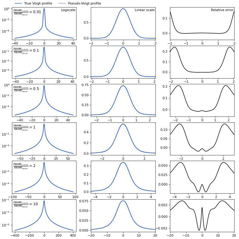
Calculating such a convolution for each spectral interval at each spatial point, given that thousands of paths are being traced, would take too much time. Therefore, I propose to replace this convolution with a weighted sum (so-called pseudo-Voigt):
with
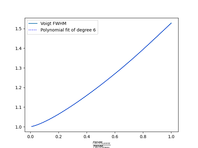
Both function, F and f can be obtained by fitting the true Voigt profile. The F function can be fitted with 6th degree polynomials of

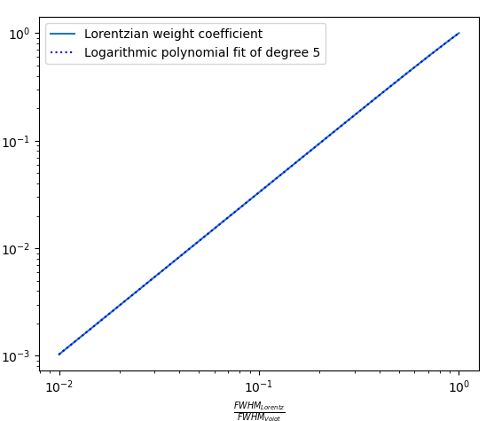
The f function can be fitted with 5th degree logarithmic polynomial of
The maximum relative error of the pseudo-Voigt approximation can reach 25%, but all the main characteristics of the spectrum: maximum intensity, FWHM, line wings are approximated well.
Here is the script that does the above fitting:
pseudo_voigt_fit.py
import numpy as np
from scipy.special import wofz
from scipy.optimize import minimize, brentq, minimize_scalar
from matplotlib import pyplot as plt


def gaussian(x, sigma):
    return np.exp(-0.5 * x**2 / sigma**2) / (sigma * np.sqrt(2. * np.pi))


def lorentzian(x, lambda_1_2):
    return (0.5 / np.pi) * lambda_1_2 / (x**2 + (0.5 * lambda_1_2)**2)


def lorentzian25(x, lambda_1_2):
    """
    Modified Lorentzian from B. Lomanowski, et al. Nuclear Fusion 55.12 (2015)
    123028, https://doi.org/10.1088/0029-5515/55/12/123028
    """
    return (lambda_1_2**1.5 / 7.47443) / (np.abs(x)**2.5 + (0.5 * lambda_1_2)**2.5)


def voigt(x, sigma, lambda_1_2):
    """
    Exact computation of Voigt profile (gauss * lorentzian) using the Fadeeva function.
    Useful to test the convolution integration.

    :param x: Function argument.
    :param sigma: Gausian sigma.
    :param lambda_1_2: Lorentzian FWHM.
    """

    z = (x + 1j * 0.5 * lambda_1_2) / (sigma * np.sqrt(2))

    return np.real(wofz(z)) / (sigma * np.sqrt(2 * np.pi))


def voigt_convolution(x, fwhm_gauss, fwhm_lorentz, mg=512, ml=64, modified_lorentzian=True):
    """
    Computes Voigt profile as a convolution of Gaussian and Lorentzian profiles.

    :param x: Function argument.
    :param fwhm_gauss: Gausian FWHM.
    :param fwhm_lorentz: Lorentzian FWHM.
    :param mg: Number of grid points per Gausian FWHM. Default: 512.
    :param ml: Number of grid points per Lorentzian FWHM. Default: 64.
    :param modified_lorentzian: Use modified Lorentzian function. Default: True.
    """

    x = np.asarray(x)
    if x.ndim == 0:
        x = x[None]
    res = np.zeros(len(x))
    m = 8 * int(max(ml * fwhm_gauss / fwhm_lorentz, mg))
    x1, dx1 = np.linspace(- 4 * fwhm_gauss, 4 * fwhm_gauss, m, retstep=True)
    sigma = fwhm_gauss / (2 * np.sqrt(2 * np.log(2)))
    f1 = gaussian(x1, sigma)
    for ix, x0 in enumerate(x):
        f2 = lorentzian25(x1 - x0, fwhm_lorentz) if modified_lorentzian else lorentzian(x1 - x0, fwhm_lorentz)
        res[ix] = (f1 @ f2) * dx1

    return res


def pseudo_voigt(x, fwhm_gauss, fwhm_lorentz, voigt_fwhm_func, weight_func, modified_lorentzian=True):
    """
    Computes pseudo-Voigt profile as a weighted sum of Gaussian and lorentzian profiles.
    F_voigt(x) = weight * F_lorentz + (1. - weight) * F_gauss

    :param x: Function argument.
    :param fwhm_gauss: Gausian FWHM.
    :param fwhm_lorentz: Lorentzian FWHM.
    :param voigt_fwhm_func: A function of fwhm_gauss and fwhm_lorentz that returns
                            approximated Voigt FWHM, fwhm_voigt.
    :param weight_func: A function of fwhm_lorentz/fwhm_voigt that returns
                        a weight of Lorentzian profile.
    :param modified_lorentzian: Use modified Lorentzian function. Default: True.
    """

    fwhm = voigt_fwhm_func(fwhm_gauss, fwhm_lorentz)
    weight = weight_func(fwhm_lorentz / fwhm)

    sigma_v = 0.5 * fwhm / np.sqrt(2 * np.log(2))
    lorentz = lorentzian25(x, fwhm) if modified_lorentzian else lorentzian(x, fwhm)
    gs = gaussian(x, sigma_v)

    return weight * lorentz + (1 - weight) * gs


def voigt_find_fwhm(fwhm_gauss, fwhm_lorentz):
    """
    Finds Voigt FWHM.

    :param fwhm_gauss: Gausian FWHM.
    :param fwhm_lorentz: Lorentzian FWHM.
    """
    fvmax = voigt_convolution(0, fwhm_gauss, fwhm_lorentz)[0]

    def root_func(x):
        return voigt_convolution(x, fwhm_gauss, fwhm_lorentz)[0] - 0.5 * fvmax

    return 2. * brentq(root_func, 0, fwhm_gauss + fwhm_lorentz, maxiter=1000)


def fwhm_polyfit(x, y, deg):
    """
    Constrained polynomial fit: a0 = 1, a1 >= 0.
    """

    def min_func(w):
        fit = 1.
        for i, w1 in enumerate(w):
            fit += w1 * x**(i + 1)

        return ((1. - fit / y)**2).sum()

    constraints = [{'type': 'ineq', 'fun': lambda w: w[0]}]

    return np.append(minimize(min_func, np.zeros(deg), constraints=constraints).x[::-1], [1.])


def pseudo_voigt_fwhm_fit(deg_gauss=6, deg_lorentz=6, n=1000):
    """
    Fits Voigt FWHM with two polynoms of given degrees.

    For FWHM_{G} <= FWHM_{L}:
        FWHM_{V} = 1. + Sum_{i=1}^{N_{G}} a_i * (FWHM_{G}/FWHM_{L})^i

    For FWHM_{G} > FWHM_{L}:
        FWHM_{V} = 1. + Sum_{i=1}^{N_{L}} b_i * (FWHM_{L}/FWHM_{G})^i

    :param deg_gauss: N_{G}
    :param deg_lorentz: N_{L}
    :param n: FWHM_{G}/FWHM_{L} and FWHM_{L}/FWHM_{G} grid sizes.

    :returns: a_i, b_i
    """

    fwhm_gauss = np.geomspace(0.01, 1, n)
    fwhm_voigt = np.zeros(n)

    for i, g in enumerate(fwhm_gauss):
        fwhm_voigt[i] = voigt_find_fwhm(g, 1.)

    poly_gauss = fwhm_polyfit(fwhm_gauss, fwhm_voigt, deg_gauss)

    fwhm_lorentz = np.geomspace(0.01, 1, n)
    fwhm_voigt = np.zeros(n)

    for i, l in enumerate(fwhm_lorentz):
        fwhm_voigt[i] = voigt_find_fwhm(1., l)

    poly_lorentz = fwhm_polyfit(fwhm_lorentz, fwhm_voigt, deg_lorentz)

    return poly_gauss, poly_lorentz


def pseudo_voigt_weight_fit(fwhm_gauss, fwhm_lorentz, voigt_fwhm_func, n, relative=True):
    """
    Fits the Lorentzian weight in the pseudo-Voigt profile.

    :param fwhm_gauss: Gausian FWHM.
    :param fwhm_lorentz: Lorentzian FWHM.
    :param voigt_fwhm_func: A function of fwhm_gauss and fwhm_lorentz that returns
                            approximated Voigt FWHM.
    :param n: The argument grid size for fitting the pseudo-Voigt profile.
    :param relative: Relative (shape) or absolute (value) fit. Default: True (relative).
    """

    fwhm_voigt = voigt_fwhm_func(fwhm_gauss, fwhm_lorentz)

    if relative:
        x = np.geomspace(0.01 * fwhm_voigt, 50 * fwhm_voigt, n)
    else:
        x = np.linspace(0, 50 * fwhm_voigt, n)
    fv = voigt_convolution(x, fwhm_gauss, fwhm_lorentz)

    fl = lorentzian25(x, fwhm_voigt)
    fg = gaussian(x, 0.5 * fwhm_voigt / np.sqrt(2 * np.log(2)))

    def fit_func(x):
        return np.abs(fv - x * fl - (1. - x) * fg).sum()

    def rel_fit_func(x):
        return ((1. - (x * fl + (1. - x) * fg) / fv)**2).sum()

    f = rel_fit_func if relative else fit_func

    result = minimize_scalar(f, bounds=(0, 1), method='Bounded')

    return result.x


n = 8192
nw = 256

poly_gauss, poly_lorentz = pseudo_voigt_fwhm_fit(deg_gauss=6, deg_lorentz=6, n=1000)

poly_gauss_func = np.poly1d(poly_gauss)
poly_lorentz_func = np.poly1d(poly_lorentz)


def voigt_fwhm_func(fwhm_gauss, fwhm_lorentz):
    if fwhm_gauss > fwhm_lorentz:
        return fwhm_gauss * poly_lorentz_func(fwhm_lorentz / fwhm_gauss)

    return fwhm_lorentz * poly_gauss_func(fwhm_gauss / fwhm_lorentz)


fwhm_lorentz = np.geomspace(0.01, 100, nw)
weight = np.zeros(nw)
fwhm_ratio = np.zeros(nw)
for i in range(nw):
    fwhm_ratio[i] = fwhm_lorentz[i] / voigt_fwhm_func(1., fwhm_lorentz[i])
    print('Step {} out of {}. Fitting lorentzian weight for FWHM_lorentz/FWHM_Voigt = {}.'.format(i + 1, nw, fwhm_ratio[i]))
    weight[i] = pseudo_voigt_weight_fit(1., fwhm_lorentz[i], voigt_fwhm_func, n, relative=True)


deg = 5
poly_weight = np.polyfit(np.log(fwhm_ratio), np.log(weight), deg)


def weight_func(fwhm_ratio):
    return np.exp(np.poly1d(poly_weight)(np.log(fwhm_ratio)))


fwhm_gauss = np.linspace(0.01, 1., 100)
fwhm_voigt = np.array([voigt_find_fwhm(fg, 1.) for fg in fwhm_gauss])
fig = plt.figure()
ax = fig.add_subplot(111)
ax.plot(fwhm_gauss, fwhm_voigt, ls='-', c='tab:blue', label='Voigt FWHM')
ax.plot(fwhm_gauss, poly_gauss_func(fwhm_gauss), ls=':', c='b', label='Polynomial fit of degree {}'.format(6))
ax.set_xlabel(r'$\frac{FWHM_{Gauss}}{FWHM_{Lorentz}}$')
ax.legend(loc=0)

fwhm_lorentz = np.linspace(0.01, 1., 100)
fwhm_voigt = np.array([voigt_find_fwhm(1., fl) for fl in fwhm_lorentz])
fig = plt.figure()
ax = fig.add_subplot(111)
ax.plot(fwhm_lorentz, fwhm_voigt, ls='-', c='tab:blue', label='Voigt FWHM')
ax.plot(fwhm_lorentz, poly_lorentz_func(fwhm_lorentz), ls=':', c='b', label='Polynomial fit of degree {}'.format(6))
ax.set_xlabel(r'$\frac{FWHM_{Lorentz}}{FWHM_{Gauss}}$')
ax.legend(loc=0)

fig = plt.figure()
ax = fig.add_subplot(111)
ax.plot(fwhm_ratio, weight, ls='-', c='tab:blue', label='Lorentzian weight coefficient')
ax.plot(fwhm_ratio, weight_func(fwhm_ratio), ls=':', c='b', label='Logarithmic polynomial fit of degree {}'.format(deg))
ax.set_xlabel(r'$\frac{FWHM_{Lorentz}}{FWHM_{Voigt}}$')
ax.set_yscale('log')
ax.set_xscale('log')
ax.legend(loc=0)

fwhm_lorentz = [0.01, 0.1, 0.5, 1., 2., 10.]

fig = plt.figure(figsize=(10., 10.), dpi=80)

for i, fwhm_l in enumerate(fwhm_lorentz):
    fwhm_v = voigt_fwhm_func(1., fwhm_l)
    x = np.linspace(-40 * fwhm_v, 40 * fwhm_v, n)
    f_voigt = voigt_convolution(x, 1., fwhm_l)
    f_pseudo = pseudo_voigt(x, 1., fwhm_l, voigt_fwhm_func, weight_func)

    ax1 = fig.add_subplot(len(fwhm_lorentz), 3, 3 * i + 1)
    ax1.plot(x, f_voigt, ls='-', c='tab:blue', label='True Voigt profile')
    ax1.plot(x, f_pseudo, ls=':', c='b', label='Pseudo-Voigt profile')
    ax1.set_yscale('log')
    ax1.text(0.02, 0.95, r'$\frac{FWHM_{Lorentz}}{FWHM_{Gauss}} = $' + '{:g}'.format(fwhm_l), va='top', transform=ax1.transAxes, fontsize=11)

    ax2 = fig.add_subplot(len(fwhm_lorentz), 3, 3 * i + 2)
    ax2.plot(x, f_voigt, ls='-', c='tab:blue', label='True Voigt profile')
    ax2.plot(x, f_pseudo, ls=':', c='b', label='Pseudo-Voigt profile')
    ax2.set_xlim(-2 * fwhm_v, 2 * fwhm_v)

    ax3 = fig.add_subplot(len(fwhm_lorentz), 3, 3 * i + 3)
    ax3.plot(x, 1. - f_pseudo / f_voigt, ls='-', c='k', label='Residual')
    ax3.set_xlim(-2 * fwhm_v, 2 * fwhm_v)

    if i == 0:
        ax1.text(0.99, 0.95, 'Logscale', ha='right', va='top', transform=ax1.transAxes)
        ax2.text(0.99, 0.95, 'Linear scale', ha='right', va='top', transform=ax2.transAxes)
        ax3.text(0.99, 0.95, 'Relative error', ha='right', va='top', transform=ax3.transAxes)
        ax1.legend(loc=2, ncol=2, frameon=False, bbox_to_anchor=(0., 1.25))

fig.subplots_adjust(left=0.05, bottom=0.03, right=0.98, top=0.97, wspace=0.23, hspace=0.18)

plt.show()
As for the Zeeman effect, I think for now we can do the same as in Lomanowski B.A. et al, namely model Stark and Zeeman effects separately (each Zeeman component is a Stark-Doppler line). Later we can try to interpolate tabular data from J. Rosato, Y. Marandet, R. Stamm, Journal of Quantitative Spectroscopy & Radiative Transfer 187 (2017) 333, where both effects are taken into account simultaneously on quantum level.